Overview
The complete paper and all appendix subsections are condensed below. Nine numbered figures, nine tables, all displayed formulas, four execution algorithms, full VLM prompts, and references are preserved. Figure 1 and its caption, absent from the HTML, are restored from the PDF.
At a glance
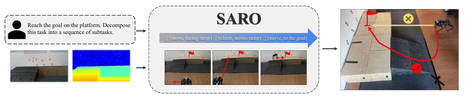
SARO combines vision-language task decomposition, a closed-loop execution state machine, and a learned quadruped controller. Probability Annealing Selection gradually replaces privileged simulated inputs with estimated latent states during locomotion training. The system crosses stairs, ramps, gaps, and doors in short navigation tasks. End-to-end reliability remains limited by localization and perceptual errors, even when the low-level controller traverses terrain successfully.
I INTRODUCTION
The goal is to connect visual reasoning about a three-dimensional route with reliable physical locomotion. The system uses pretrained VLM inference for a restricted action vocabulary and geometric controllers for execution, rather than directly asking the VLM for joint commands. PAS addresses the mismatch between a privileged training policy and a deployed proprioception-only controller. Experiments intentionally use one connecting terrain feature per task because the front-facing view and memory-free design limit longer planning.
II RELATED WORKS
II-A Foundation Models in Robotics
Prior foundation-model systems translate commands, propose visual navigation actions, or combine language reasoning with robot skills. This work emphasizes simple routes that require crossing a change in terrain or a doorway. Its broad criticism of earlier systems motivates that setting; the experiments do not establish superiority over every prior navigation formulation.
II-B Locomotion Control of Quadruped Robots
Learning-based locomotion commonly exploits privileged simulation information, then adapts or distills to deployable observations. SARO instead continues reward-driven optimization while progressively substituting a recurrent estimator’s latent output for the privileged latent. This retains privileged training support without relying solely on imitation in the second stage.
III METHOD
III-A Task Definition
A task contains two platforms connected by one stair, ramp, gap, or door. The robot starts on the first and receives both a target position/yaw relative to its starting pose and a language description of the goal on the second. Thus the system has a specified geometric goal, rather than solving unrestricted language-only exploration. The full navigation stack uses onboard RGB, depth, inertial, and joint information; only its low-level locomotion actor is proprioception-only.
Equation
III-B High-level Reasoning and Task Execution
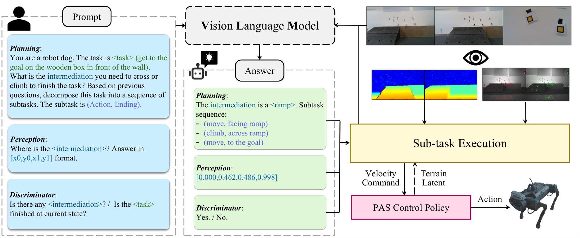
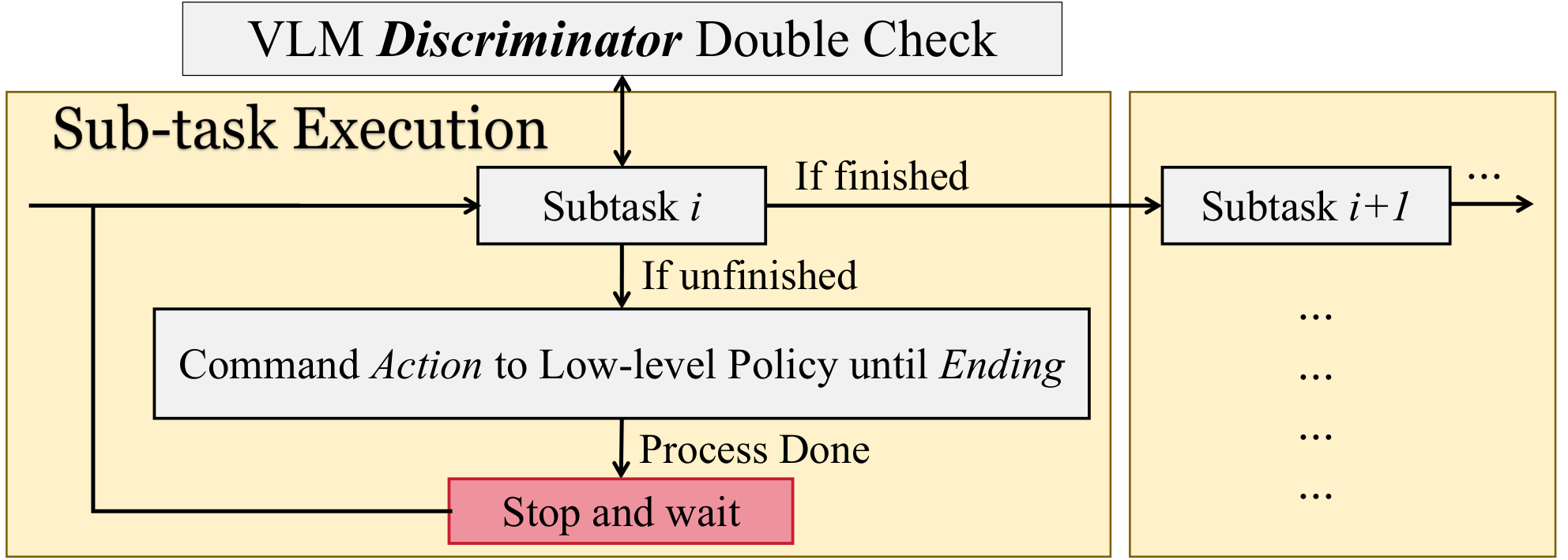
LLaVA decomposes the task into action/ending pairs. Actions are move or climb; endings describe facing the connector, crossing it, or reaching the goal. A predefined controller turns each pair into velocity commands using VLM localization, aligned depth, and odometry. Before moving to the next subtask, a VLM discriminator checks completion. Repeated execution and checking can correct an initially incomplete alignment or crossing. This is a designed state machine with visual feedback, not a learned general planner or a formal safety guarantee.
III-C Low-level Locomotion Control Policy
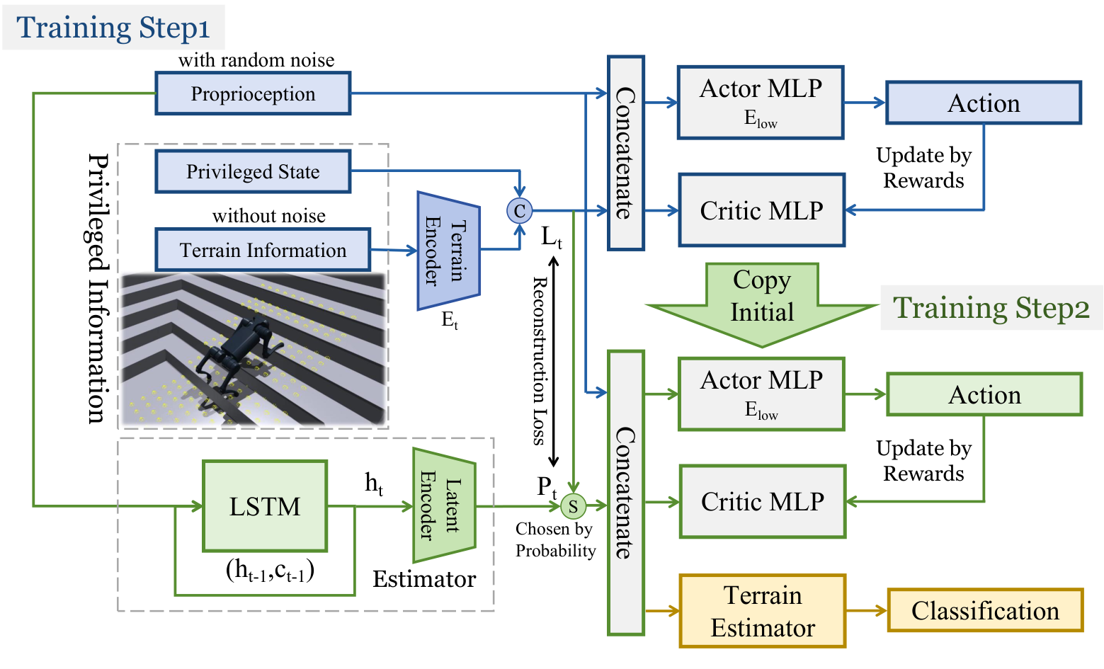
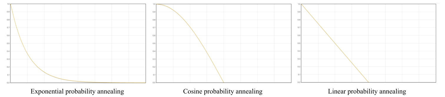
Stage one trains an oracle actor from 45 proprioceptive values, four privileged state values, and 187 terrain heights. A terrain encoder compresses heights to 32 values; adding the privileged state yields a 36-dimensional latent and an 81-dimensional actor input. The critic uses the full 236-dimensional observation. A recurrent estimator simultaneously learns to reconstruct the privileged latent. Stage two initializes from these networks and jointly optimizes the estimator and actor with reinforcement learning. PAS initially supplies mostly true latents, then selects estimated latents with increasing probability until deployment uses only estimates. Selection is applied across robots to preserve consistency within continuous behavior. The actor outputs twelve desired joint positions.
Equations 1–4
| (1) | ||||
| (2) | ||||
| (3) | ||||
| (4) |
IV EXPERIMENTS
IV-A Experiment Setup
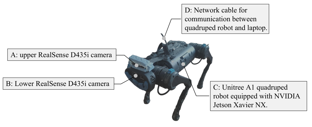
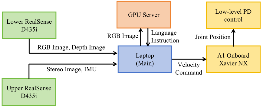
The Unitree A1 runs its controller at 50 Hz on a Jetson Xavier NX. Two RealSense D435i cameras supply separate visual-inertial odometry and RGB-D reasoning views. A laptop runs VINS-Fusion and the main state machine; an external server with eight RTX 3090 GPUs runs LLaVA-34B [61]. ROS carries images, language outputs, velocity commands, and joint targets. Laboratory wall decorations provide visual features to stabilize odometry. The complete system therefore depends on external computation and communication, despite onboard sensing and low-level control.
IV-B Results of High-level Reasoning
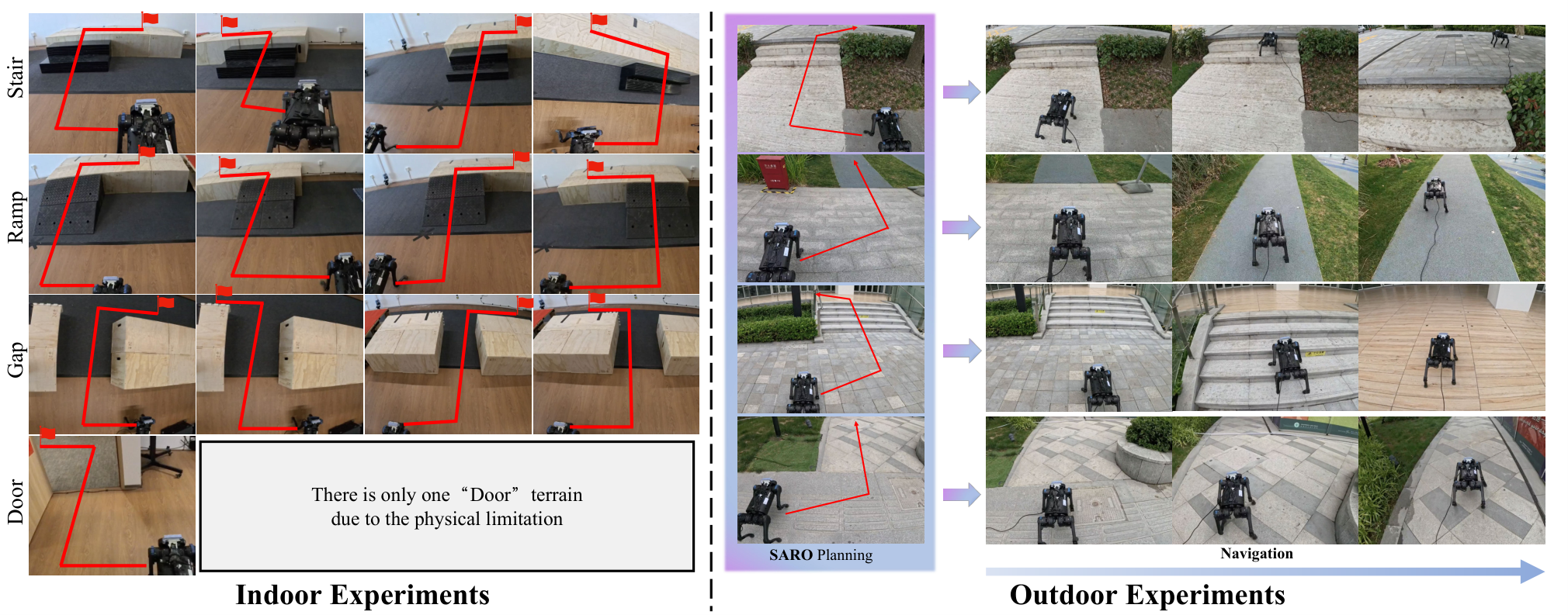
Twenty trials per terrain evaluate indoor navigation. Overall success is 60% for stairs, 25% for ramps, 45% for gaps, and 30% for doors. Terrain-crossing-only success is higher at 70%, 50%, 80%, and 50%; the separately reported stable-localization results are 88%, 67%, 94%, and 63%. These columns measure different conditions and should not be conflated. Removing closed-loop checking reduces overall success to 10–20%. The tested ViNT and small LSTM baselines score zero in all four settings; NoMaD scores 20% on gaps and 70% on doors, exceeding SARO on the door task. Baselines use different navigation interfaces, and the LSTM learns from only fifty short recorded trajectories, so these comparisons establish performance on this setup rather than general model rankings. Motion blur and tilted views degrade localization, especially on ramps. Outdoor examples illustrate transfer but provide no separate aggregate outdoor success table.
| Intermediation | Overall | Stable Loc | w/o Closed-Loop | NoMaD | LSTM | Across Terrains | ViNT |
|---|---|---|---|---|---|---|---|
| Stair | 60% | 88% | 10% | 0% | 0% | 70% | 0% |
| Ramp | 25% | 67% | 10% | 0% | 0% | 50% | 0% |
| Gap | 45% | 94% | 20% | 20% | 0% | 80% | 0% |
| Door | 30% | 63% | 15% | 70% | 0% | 50% | 0% |
IV-C Results of Low-level Locomotion
Simulation uses 4,096 runs per terrain. A run counts as successful if it reaches a terrain edge or merely remains alive for twenty seconds, so simulated success is not always completed traversal. PAS averages 85.31% success, compared with 77.34% for direct blind training, 70.40% for concurrent estimation, 58.05% for action imitation, and 49.30% for RMA. Exponential selection decay with base 0.9998 gives the best displayed averages; the competing schedules are close in success but differ more in tracking scores. Physical locomotion evaluates twenty trials per terrain and requires reaching the end without falling or getting stuck. PAS reports 100% on stairs, 90% on ramps, 95% on rubble, 100% on grassland, and 95% on unseen obstacles. These controller-only results are substantially better than the full navigation results because they do not test the same perception, localization, and goal-completion pipeline.
| Metric | PAS(ours) | RMA[1] | IL[55] | Blind | Concurrent[64] |
|---|---|---|---|---|---|
| SR (Avg) | 85.31% | 49.30% | 58.05% | 77.34% | 70.40% |
| L vel (Avg) | 0.8790 | 0.6848 | 0.8029 | 0.8555 | 0.8330 |
| A vel (Avg) | 0.7815 | 0.5895 | 0.7370 | 0.7627 | 0.7349 |
| Metric | Exp 0.9998 | Exp 0.9995 | No anneal | Cosine | Linear |
|---|---|---|---|---|---|
| SR (Avg) | 85.31% | 83.60% | 83.33% | 83.26% | 84.00% |
| L vel (Avg) | 0.8790 | 0.8710 | 0.8687 | 0.8730 | 0.8715 |
| A vel (Avg) | 0.7815 | 0.7741 | 0.7733 | 0.7466 | 0.7660 |
V CONCLUSION
A restricted visual state machine and a transferable locomotion policy can cooperate on short terrain-crossing tasks. Localization instability, vibration, image blur, limited field of view, and absent persistent memory constrain end-to-end reliability. The authors propose improved perception and topological or semantic maps for more complex routes. The current evidence supports the tested simple tasks rather than unrestricted long-horizon navigation.
APPENDIX
The appendix documents the exact prompts, four execution routines, locomotion training specification, and additional evaluation definitions. All technical tables and pseudocode are retained.
V-A Details of High-level Reasoning and Task Execution
V-A 1 VLM Details and Prompts
LLaVA-34B receives 848×480 images. Planning selects the connector and a sequence of allowed subtask pairs; perception asks for its bounding box; discrimination checks visibility or completion. After planning, the identified connector replaces the prompt placeholder. The original three prompt templates follow so the restricted interface can be reproduced.
- 1.
Planning “Ignore anything on the wall. You are a robot dog. The intermediation may be a stair, a ramp, a gap, or a door frame. The task is task. First answer the question: 1. What is the only intermediation you need to cross or climb to finish the task? Based on previous questions, decompose this task into a sequence of subtasks. The subtask is (Action, Ending). Action is one of [‘move’, ‘climb’]. The ending is one of [‘facing intermediation’, ‘across intermediation’, and ‘to the goal’]. Replace the intermediation with the answer to question 1.”
- 2.
Perception “Where is the intermediation? Answer in [x0,y0,x1,y1] format, don’t say anything else.”
- 3.
Discriminator “Is there any intermediation? Just answer yes or no.” or “Is the task finished at current state?”
V-A 2 Sub-task Set and Deployment Details
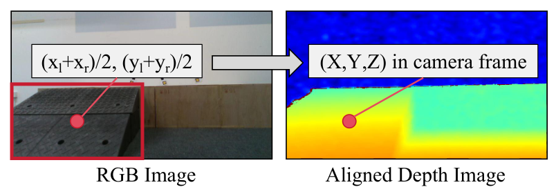
Four pairs are used: move to face the connector, move across it, move to the goal, and climb across it. Alignment combines a VLM box with depth and a camera projection; position controllers use a 0.1 m tolerance. Climbing uses transitions between flat-terrain and crossing predictions, followed by the visual completion check. The pseudocode preserves source inconsistencies that need resolution in implementation: Algorithm 1 reuses center-coordinate symbols in its projection and threshold, while Algorithm 4 initializes TerrainChangeCount but updates Count and does not explicitly show the previous-class update. The stated projection assumes calibrated camera geometry; VLM boxes and depth do not guarantee an exact physical target.
V-B Training Details of Low-level Locomotion Control Policy
Training uses IsaacGym with 4,096 parallel robots, PPO [66], a 0.02-second control step, and 40,000 iterations in each of the two stages.
V-B 1 Problem Definition
Proprioception comprises gravity direction, base angular velocity, commanded planar/angular velocity, joint positions and velocities, and the previous action. Privileged information supplies base linear velocity and ground friction; the terrain grid supplies 187 heights. Deployment cannot reliably obtain the privileged linear velocity by integrating inertial acceleration because drift accumulates. Desired joint positions pass to proportional-derivative controllers with gains 40 and 0.5. The appendix’s naming reuses the same symbol for proprioception and the estimated latent, but their dimensions and roles differ.
V-B 2 Reward Function
Rewards combine exponential linear/angular velocity tracking, a per-step survival bonus, penalties for energy, joint motion and base angular instability, and gait-style terms for foot airtime and force balance. Table V retains every formula and weight. These shaped objectives encourage tracking and stable gait but are not themselves task-level navigation success measures.
| Type | Item | Formula | Weight |
|---|---|---|---|
| Task | Lin vel | ||
| Ang vel | |||
| Safety | Alive | 1 | |
| Performance | Energy | ||
| Joint vel | |||
| Joint acc | |||
| Ang vel Stability | |||
| Style | Feet in air | ||
| Balance |
V-B 3 Termination Conditions
Episodes terminate after excessive roll above 0.8 radians, pitch above 1.0 radian, or lack of significant motion for over one second. Reaching an edge or surviving twenty seconds also ends the episode as a timeout. The source incorrectly describes pitch as rotation about the vertical axis; the stated roll/pitch thresholds are retained without repeating that axis error.
V-B 4 Terrain Curriculum
The curriculum contains eighty 8 m×8 m terrains: ten difficulty levels in each of eight categories. Ascending/descending stairs reach 0.2 m height with 0.3 m treads; ascending/descending platforms range from 0.16 to 0.22 m high and 0.8 to 1.5 m wide. Ascending/descending ramps reach 30 degrees. Flat ground and Perlin-noise rough ground, up to 0.15 m amplitude, complete the set. Progressive difficulty supports early training stability.
V-B 5 Dynamic Randomization
Randomization varies mass, center-of-mass position, initial joints and velocity, motor strength, and friction. Gaussian noise perturbs observations, velocity commands change every five seconds, and external disturbances occur every nine seconds. Tables VI and VII preserve the numeric ranges and amplitudes; the table’s base-mass range is reproduced as given rather than interpreted as a complete physical robot mass.
| Parameters | Range | Unit |
|---|---|---|
| Base mass | [0, 3] | |
| Mass position of X axis | [-0.2, 0.2] | |
| Mass position of Y axis | [-0.1, 0.1] | |
| Mass position of Z axis | [-0.05, 0.05] | |
| Friction | [0, 2] | - |
| Initial joint positions | [0.5, 1.5]nominal value | |
| Initial base velocity | [-1.0, 1.0] (all directions) | |
| Motor strength | [0.9, 1.1]nominal value | - |
| Observation | Gaussian Noise Amplitude | Unit |
|---|---|---|
| Linear velocity | 0.05 | |
| Angular velocity | 0.2 | |
| Gravity | 0.05 | |
| Joint position | 0.01 | |
| Joint velocity | 1.5 |
V-B 6 Terrain Classification
After PAS training, policy weights are frozen and a binary cross-entropy head learns flat-versus-connector classification. A reproduction ambiguity remains: the appendix and architecture table list privileged and terrain inputs for this classifier, while the main deployment claim emphasizes proprioceptive inference. The source does not clearly reconcile the classifier’s deployable inputs.
V-B 7 Network Architecture
The terrain encoder and actor are multilayer perceptrons. The estimator combines an LSTM with an MLP, using recurrent history to infer unobserved terrain/state information. Table VIII retains all hidden-layer sizes, the critic, and the added terrain head. Its listed actor inputs should be read alongside the main architecture’s encoded latent pathway.
V-B 8 Hyperparameters
Table IX preserves PPO settings, including learning rate 0.001, discount 0.99, advantage parameter 0.95, clip parameter 0.2, entropy coefficient 0.01, four minibatches, and twenty-four rollout steps per environment.
| Hyperparameter | Value |
|---|---|
| clip min std | 0.05 |
| clip param | 0.2 |
| desired kl | 0.01 |
| entropy coef | 0.01 |
| gamma | 0.99 |
| lam | 0.95 |
| learning rate | 0.001 |
| max grad norm | 1 |
| num mini batch | 4 |
| num steps per env | 24 |
V-C Extra Experiments Details of the Low-level Locomotion
V-C 1 Metric of Velocity Tracking Ratio
The so-called tracking ratios are exponential transforms of squared planar or yaw-rate error, scaled by 0.25. They approach one for accurate tracking and decline with error; they are not the literal ratio of attained speed to commanded speed. Both exact formulas are retained.
Equation
| Linear velocity tracking ratio | |||
| Angular velocity tracking ratio |
V-C 2 Comparison Experiments
RMA uses an asynchronous adaptation module; imitation learning retains the first-stage teacher and learns an action-level student; the built-in A1 MPC appears only in physical comparisons. The blind baseline trains the deployable recurrent architecture directly from proprioception. Concurrent training learns a state estimator alongside the policy without terrain inputs. These variants isolate different uses of privileged information, supervision, and staged training.
V-C 3 Ablation Experiments
The ablation compares exponential bases 0.9998 and 0.9995, immediate estimated-latent use without annealing, cosine decay, and linear decay. Figure 9 retains all three schedule plots. The slower exponential schedule performs best on the reported averages, but the results establish an empirical choice for this training setup rather than a general optimal annealing rule.