At a glance
GCS* extends heuristic graph search to graphs whose vertices contain continuous convex decision sets and whose edges couple those decisions. A cheapest path to a vertex need not reach the points needed to continue, so keeping only that path can lose both feasibility and optimality. GCS* instead keeps paths that reach some terminal point more cheaply, or that reach a previously unreachable point.
Conservative containment checks preserve completeness and, with a pointwise admissible heuristic and cost-based pruning, optimality. Faster sampled checks can wrongly prune useful paths; their guarantees are probabilistic or asymptotic. In three simplified planar-pushing tasks, even one sample per check works well. This is empirical evidence under a translation-only, frictionless model, not a finite-sample optimality guarantee or a physical-robot evaluation.
1 Introduction
A graph of convex sets separates discrete mode choices from continuous variables within each mode. Edge constraints enforce relationships such as trajectory continuity. Fixing a discrete path leaves a convex program, but choosing the path is generally NP-hard and enumerating every mode can be infeasible.
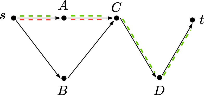
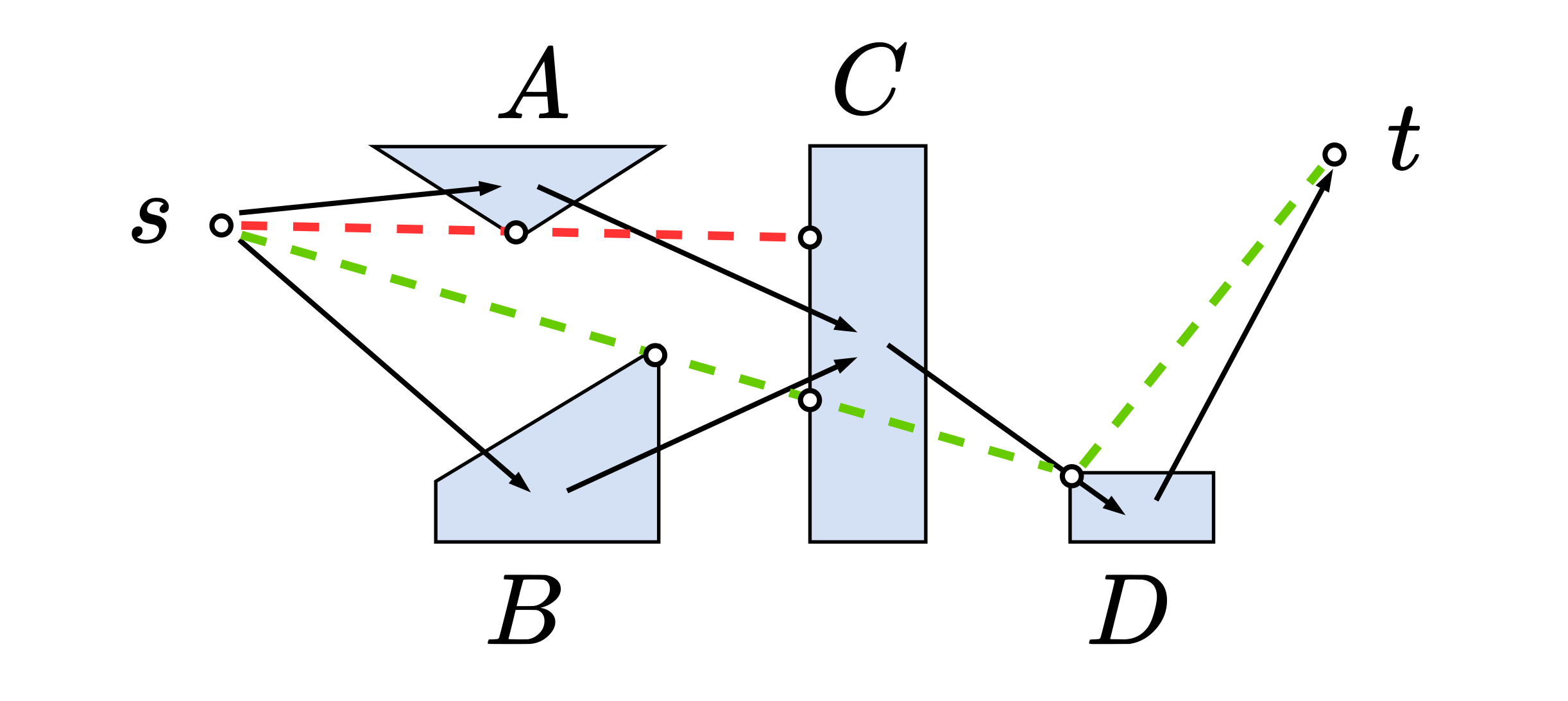
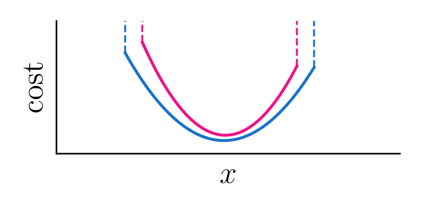
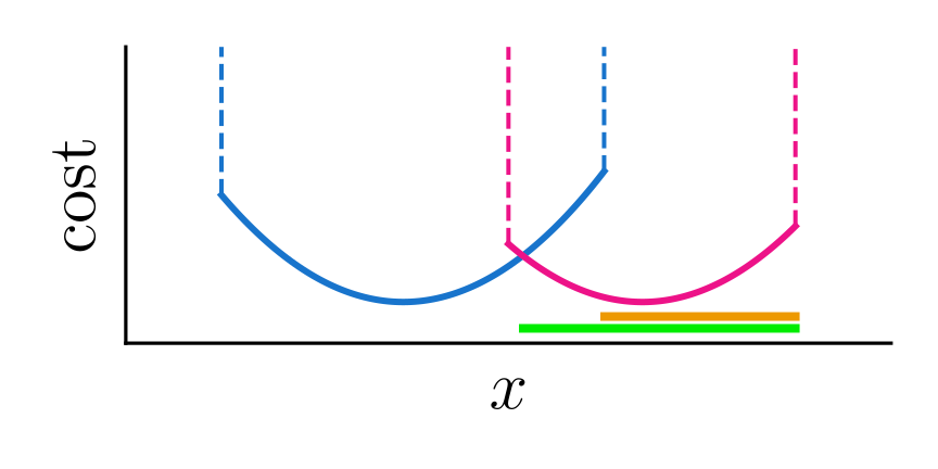
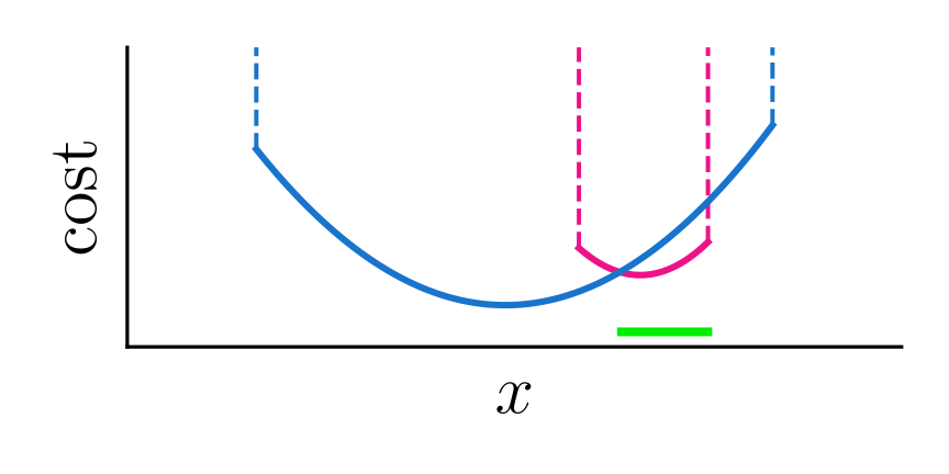
Unlike ordinary A*, a GCS solver cannot safely discard a path merely because another reaches the same vertex with lower scalar cost. Figures 2–3 show why: the paths may reach different continuous points, and only the more expensive one may permit continuation. Optimal substructure survives at the trajectory-point level. The formulation allows repeated vertices, because returning to a set at a different point may be useful.
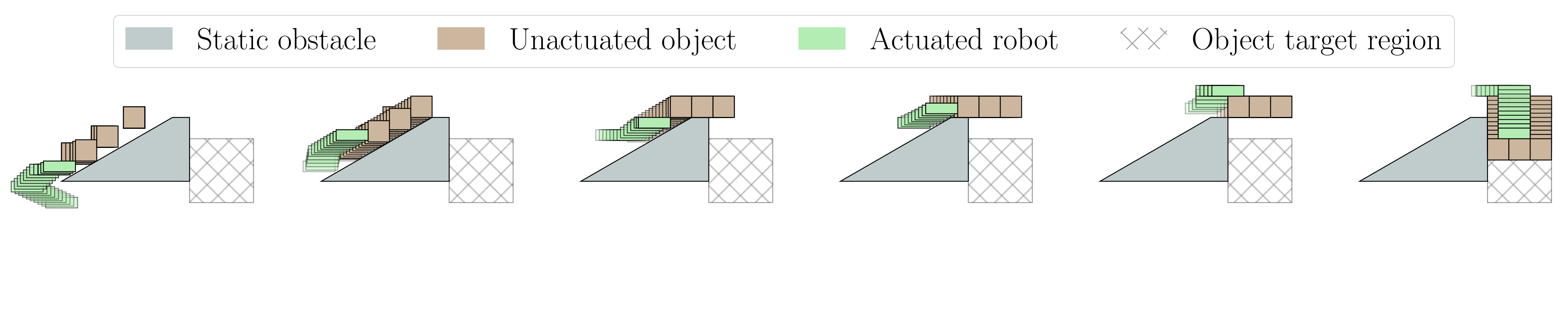
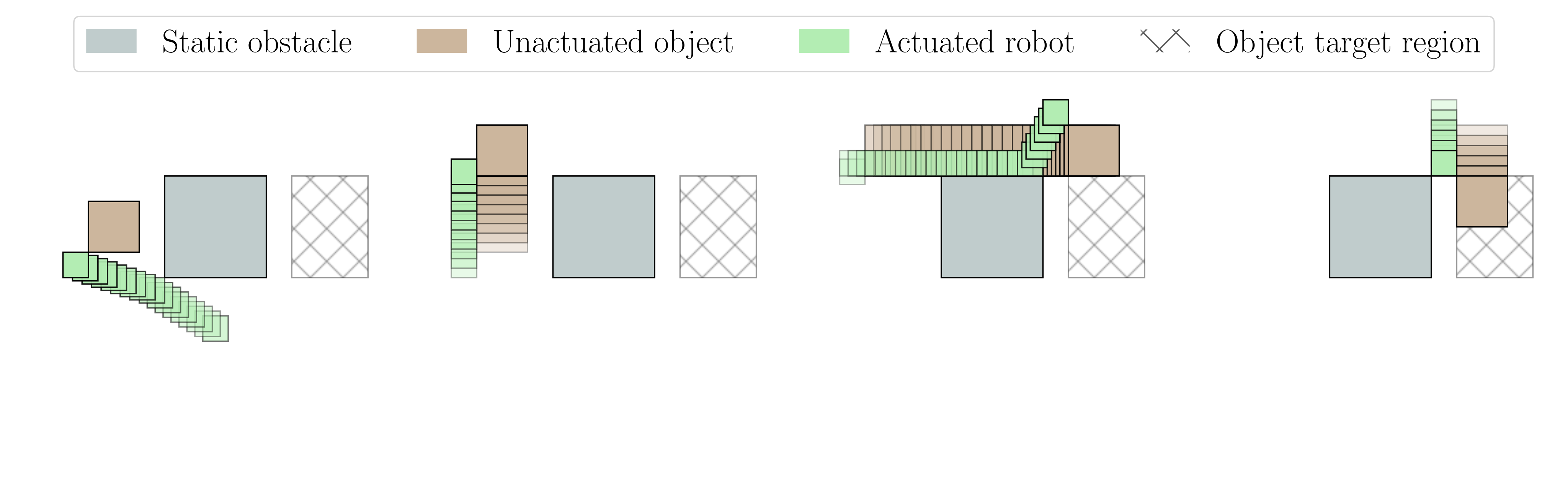
GCS* uses an implicit successor operator and retains multiple paths per vertex. ReachesCheaper preserves any path that improves cost at some terminal point; ReachesNew retains only paths that expand terminal reachability. The latter trades optimality for more aggressive pruning. Figure 1 illustrates a 21.9-second sampled, inflated-heuristic solution on a nominal billion-vertex graph.
2 Related Work
Sampling planners handle large spaces but face difficulties with coupled continuous constraints. Whole-problem mixed-integer convex optimization and GCS relaxations give strong continuous reasoning but require an explicit graph. Logic-geometric planning combines search and nonconvex optimization, whose local solves do not establish the same global guarantees.
IxG and IxG* also interleave graph search and optimization. The comparison here emphasizes jointly infeasible edge constraints and the cost of precomputing heuristics on an explicit graph. IxG can lose completeness in that setting; IxG* remains complete but may prune poorly when its preliminary search supplies no finite solution bound. GCS* replaces that dependence with path-domination checks.
3 Problem Formulation
Each vertex has a compact convex set, each edge has closed convex coupling constraints, and each vertex has finitely many successors. Edge costs are proper, closed, convex, positive, and bounded away from zero in the general analysis. The graph may be infinite and paths may revisit vertices.
Program 1 jointly chooses a vertex sequence and a continuous trajectory, minimizing summed edge costs under membership, successor, and edge constraints. Table 1 retains the notation. Once the vertex sequence is fixed, ConvexRestriction computes its feasible optimal trajectory. The later pushing implementation uses a zero-cost final edge into the terminal set as a special case; its ordinary mode transitions retain a positive unit penalty.
| Directed graph with vertices and edges | |
| Convex set associated with vertex | |
| Convex constraint set for edge | |
| Source and target vertices | |
| Discrete path in the graph, defined as a sequence of vertices | |
| The -th vertex in the path | |
| Last vertex in the path | |
| Set of edges traversed by path | |
| Continuous trajectory | |
| The -th point on trajectory | |
| The point on trajectory associated with vertex | |
| Cost of the edge between vertices and , evaluated on trajectory | |
| Optimal cost of a solution via vertex | |
| Optimal cost-to-come from to point | |
| Optimal cost-to-go from point to | |
| Total cost estimate via path | |
| Total cost estimate via path and point | |
| Optimal cost-to-come from to point via path | |
| Heuristic estimate of cost-to-go from point to | |
| Optimal trajectory via path subject to the heuristic |
Equations 1a–1e
| (1a) | ||||||
| (1b) | ||||||
| (1c) | ||||||
| (1d) | ||||||
| (1e) | ||||||
4 Approach
The search combines convex optimization of partial paths with either cost-based or reachability-based domination. Its queue priorities and pruning tests have different roles: a favorable priority alone does not justify discarding other ways to reach a continuous set.
4.1 Graph Search Formulation
Algorithms 1–2 contrast ordinary A* with GCS*. Both expand the lowest estimated total-cost path. Ordinary A* stores one best path per terminal vertex; GCS* stores a set of retained paths and adds a candidate only when NotDominated accepts it.
A partial path’s priority minimizes cost-to-come plus the heuristic over the points it can reach. Fixing a particular terminal point gives a more constrained value used in domination checks. A convex heuristic permits these quantities to be evaluated through ConvexRestriction. The heuristic is nonnegative; cost optimality additionally requires pointwise admissibility over each vertex set, as stated in Definition 1. The retained formulas distinguish optimal cost functions from computational estimates.
Equation
Equation
Definition 1
A heuristic function is pointwise admissible if
Equation
4.2 Domination Checks
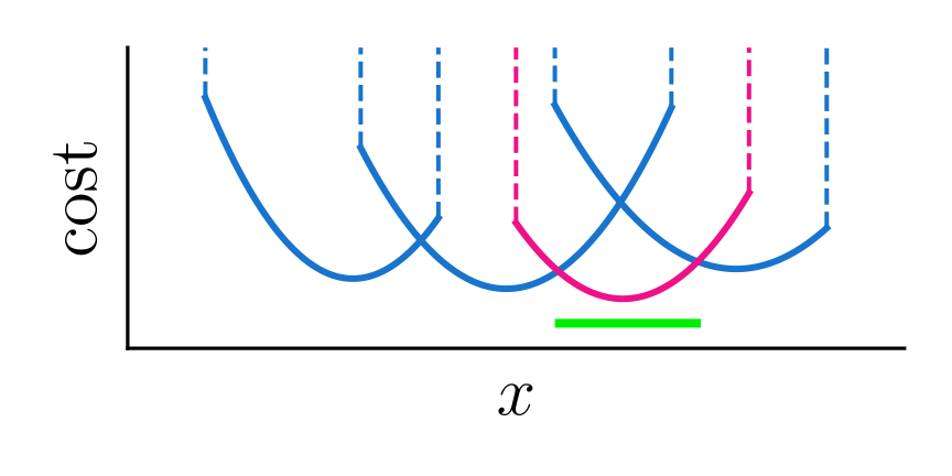
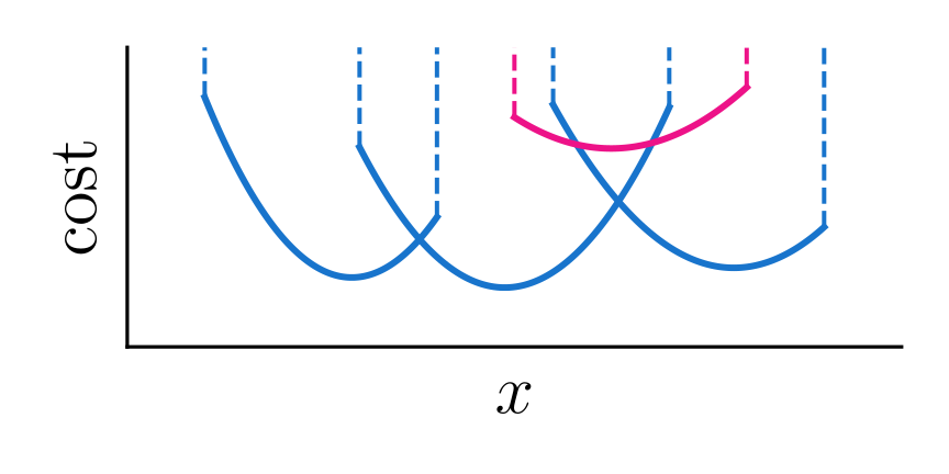
ReachesCheaper is true when some reachable terminal point costs strictly less through the candidate than through every retained alternative. ReachesNew is true when the candidate reaches a point none of those alternatives can reach. New reachability implies cheaper reachability, but a cheaper path can cover only already reachable points.
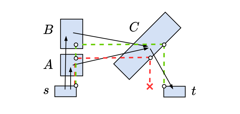
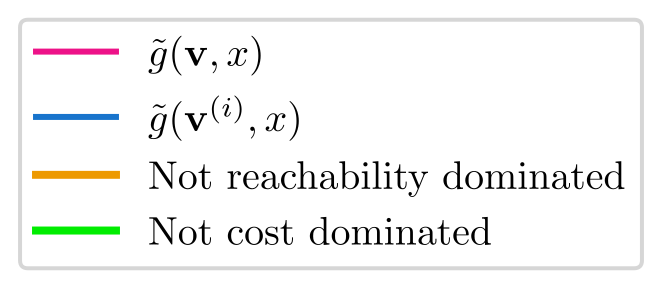
A conservative check may retain unnecessary paths but never falsely declares a useful candidate dominated. Conservative ReachesNew preserves the existence of feasible continuations; conservative ReachesCheaper also preserves the paths needed for an optimum. Figure 4 distinguishes domination by one path from domination by several paths collectively.
Equations 2–3
| (2) | ||||
| (3) | ||||
Sampling-based Approximation.
Sampling tests the defining conditions at selected terminal points. Finding one witness proves that the candidate should be retained. Failing to find a witness does not prove domination: a small region where the candidate is useful may be missed. These checks can therefore discard a necessary or cheaper path at any finite sample budget.
Polyhedral-containment-based Approximation.
The reachable set is the projection of all feasible trajectories onto the terminal variables. Cost domination uses the corresponding epigraph of optimal cost-to-come. Exact pruning asks whether the candidate’s set lies inside the union of the alternatives’ sets, which is generally nonconvex and difficult.
The implementation instead tests containment by one alternative at a time and uses a sufficient polyhedral-containment certificate. Successful containment safely prunes a candidate; failure can retain a dominated candidate. This conservatism preserves the relevant guarantees but increases work. The tested polyhedral sets and linear costs fit this certificate directly; more general convex models require additional approximation machinery. Equations 6a–b, absent from the HTML, are restored from the matching PDF.
Equations 4a–5b
| (4a) | |||
| (4b) | |||
| (4c) |
| (5a) | |||
| (5b) |

4.3 Properties of the Algorithm
Under conservative domination checks, finite branching, the cost assumptions, and suitable priorities, a feasible solution is reached in finitely many iterations. With conservative ReachesCheaper and a pointwise admissible heuristic, the returned solution is cost optimal. The exact theorem statements are retained below.
An infeasible problem can still run forever when the graph is infinite or cycles are allowed. A maximum path length restores finite failure detection for that bounded problem. Inflating an admissible heuristic trades speed for bounded suboptimality under the corresponding conservative cost-based search; finite sampled pruning does not provide the same deterministic bound.
Theorem 4.1
GCS* returns a path from to in finite iterations if one exists.
Efficiency.
GCS* is not optimally efficient in the A* sense. Expanding a partial path reveals stronger information about future cost, but this implementation does not use that information to update its heuristic. Multiple paths ending in the same set can consequently be expanded even when a more sophisticated method might avoid them.
Properties when using sampling-based domination checks.
The sampling argument takes the number of samples per domination check to infinity. The authors reason that an uncovered region is relatively open within the reachable set and, when nonempty with positive sampling probability, is eventually encountered. Thus completeness and cost optimality are limiting properties under the relevant sampling and heuristic assumptions.
This statement concerns increasing coverage per check; simply allowing a run with a fixed one-sample pruning rule to continue does not repair a path already discarded. The experiments use projected samples, and their strong finite-sample performance is a property observed in these tasks.
5 Application to Planar Pushing
Planar pushing provides an intentionally combinatorial test: each pair of bodies can have different contact and separation modes. The authors aim to demonstrate search over a huge implicit graph, rather than establish the strongest possible manipulation planner. Hierarchy or more careful mode enumeration could reduce this particular search space.
5.1 Formulation
Polyhedral robots and objects translate without rotation among static obstacles. Contacts are frictionless, and quasi-static velocities are proportional to net forces. A vertex stores two position knots for each moving body, robot actuation forces, and contact-force magnitudes. Changing one pair’s contact state or separating face generates successors on demand.
All tested constraints are linear. Rotations, frictional contact, and more general shapes would need a richer formulation or relaxation. An approximate free-space decomposition may miss contact boundaries or be expensive to generate online, so the simple successor construction does not automatically transfer to arbitrary robot configuration spaces.
Non-penetration.
For each body pair, one polyhedral face acts as a separating hyperplane. Requiring the bodies to remain on opposite sides enforces non-penetration within that convex mode.
Contact.
A body pair may be separated, in face–face contact, or in face–vertex contact. Each active contact adds a normal force and position constraints. Sliding along the contacting features is allowed while contact remains feasible; tangential friction forces are omitted.
Quasi-static dynamics.
Between consecutive knots, each body’s translation is proportional to its summed forces, including actuation for robots. Edge constraints equate the preceding mode’s final positions with the next mode’s initial positions. Feasibility therefore depends on a common continuous configuration, not only a legal sequence of mode labels.
5.2 Implementation Details
Two knots per mode give an L1 displacement cost with unit weights for all moving bodies, plus a unit mode-switch penalty. The terminal edge costs zero. The shortcut heuristic ignores contact dynamics and downweights robot displacement to 0.2; an additional mode penalty accounts for at least one further switch when no direct target edge exists. Faster runs inflate this heuristic by ε = 10.
Each sampled domination check uses one point, drawn in the terminal set and projected onto the path’s reachable set. Containment checks first try this cheap witness and run the certificate only if it fails. The implementation exploits this model’s structure by comparing final position knots rather than every force variable, and eliminates equality constraints through a null-space parameterization. These optimizations are specific to the modeled dynamics.
Equations
6 Results
AROUND has 194 vertices and 8,328 edges; SQUEEZE has 628 vertices and 56,806 edges. STACK has five bodies, approximately 1.3 billion vertices, and up to 8.5×10¹⁷ edges. Set dimensions range from 4–12 in the smaller tasks and 8–24 in STACK. Table 2 reports runtime, cost, and expanded paths on an AMD Ryzen 9 7950X; the paper does not report repeated-run uncertainty.
Sampled ReachesCheaper with the admissible heuristic solves AROUND in 26.2 seconds at cost 27.5 and SQUEEZE in four minutes at 47.80; STACK reaches the ten-hour cutoff. With ε = 10, the same check solves all three in 2.9, 38.3, and 21.9 seconds, with costs 27.5, 54.55, and 67.53. Thus the fastest SQUEEZE result sacrifices cost, and STACK’s fast finite-sample result is not a demonstrated exact optimum.
Sampled ReachesNew takes 2.5, 20, and 21.8 seconds, with SQUEEZE cost increasing to 57.42. Conservative containment preserves stronger guarantees but scales poorly: admissible ReachesCheaper takes 7.5 hours even on AROUND. Conservative ReachesNew is faster than the cost-based certificate, solving STACK in 3.5 minutes.
IxG requires 1.1 minutes of preprocessing for AROUND and 1.7 hours for SQUEEZE before the query times shown. It solves AROUND but fails on SQUEEZE; IxG* reaches the ten-hour cutoff in these tests. Neither baseline can construct STACK’s graph for its required heuristic preprocessing. These comparisons support the benefit of implicit, query-focused search on the chosen formulation.
The authors attribute effective one-sample pruning to the restrictive final object/robot configurations in these problems. That explanation and three task results do not establish comparable coverage in arbitrary high-dimensional graphs. Figures 1 and 5 retain all trajectory snapshots; videos are linked from the project page.

| Alg. | DC | Impl. | Heur. | Com- plete | Cost optimal | AROUND | SQUEEZE | STACK | ||||||
| Time | Cost | Exp | Time | Cost | Exp | Time | Cost | Exp | ||||||
| GCS* | RC | Sampl. | Admiss. | Yes† | Opt.† | 26.2s | 27.5 | 432 | 4m | 47.80 | 2114 | |||
| GCS* | RC | Cont. | Admiss. | Yes | Opt. | 7.5h | 27.5 | 734 | ||||||
| IxG* | N.A. | N.A. | Admiss. | Yes | Opt. | - | - | - | ||||||
| GCS* | RC | Sampl. | Inadm. | Yes† | -subopt.† | 2.9s | 27.5 | 51 | 38.3s | 54.55 | 381 | 21.9s | 67.53 | 57 |
| GCS* | RC | Cont. | Inadm. | Yes | -subopt. | 4.6m | 27.5 | 73 | ||||||
| IxG* | N.A. | N.A. | Inadm. | Yes | -subopt. | - | - | - | ||||||
| GCS* | RN | Sampl. | Inadm. | Yes† | Subopt. | 2.5s | 27.5 | 44 | 20s | 57.42 | 259 | 21.8s | 67.53 | 57 |
| GCS* | RN | Cont. | Inadm. | Yes | Subopt. | 35.4s | 28.5 | 75 | 20.5m | 57.42 | 458 | 3.5m | 67.53 | 64 |
| IxG | N.A. | N.A. | Inadm. | No | Subopt. | 4.7s | 28 | 31 | 2.3m | Fail | 615 | - | - | - |
7 Conclusion
GCS* makes forward search compatible with continuous sets by testing terminal reachability and pointwise cost, rather than one scalar cost per vertex. It offers conservative guarantees or faster sampling approximations, with a substantial gap in practical runtime between them. Richer contact dynamics, rotations, stronger heuristics, hierarchy, and factorization remain future directions.
Acknowledgements
Support came from the Aker Scholarship, Amazon, The AI Institute, the Army Research Office, and the Charles Stark Draper Laboratory. Rebecca H. Jiang is a Draper Scholar.
Disclosure of Interests.
The authors declare no competing interests relevant to the article.
Appendix 0.A Proofs of Algorithmic properties
Appendix A proves feasible-case completeness for conservative reachability-preserving checks and optimality for conservative ReachesCheaper with a pointwise admissible heuristic. The exact statements are retained; the proofs below give their main argument. Infeasible-case termination requires the path-length bound described in the main text.
Completeness.
Lemma 1 establishes eventual queue expansion: positive transition-cost bounds and finite branching leave only finitely many paths below a fixed finite priority. A queued feasible path is therefore expanded eventually, unless a solution is returned first.
Lemma 2 follows a feasible trajectory to its furthest point reached by any queued path. Expanding a path reaching that point must either add a continuation or find that an existing path already reaches the next point. Conservative pruning cannot remove every continuation. Combining the two lemmas gives finite discovery and return of a feasible target path.
Lemma 1
For any path in , GCS* either expands after a finite number of iterations or returns a feasible path to the target first.
Lemma 2
If target is reachable from source , then some path that reaches it is added to in finite iterations.
Theorem 0.A.1
GCS* returns a path from to in finite iterations if one exists.
Cost-optimality.
Lemma 3 follows an optimal trajectory. Before reaching the target, the queue retains a path attaining optimal cost to some point on it: if an extension is pruned, an existing path must already reach that point at least as cheaply. Pointwise admissibility then bounds some queued priority by the global optimum, as shown in the retained inequality chain.
The final contradiction is the A* argument at the point level. At a target, the nonnegative admissible heuristic is zero. Returning a more expensive target would require popping it ahead of the queued path whose estimated cost does not exceed the optimum, contradicting the queue order. This proof depends on conservative cost pruning and does not directly certify the one-sample experimental variant.
Lemma 3
Suppose prog. (1) is feasible and is an optimal path from to . If is unexpanded, there is a path in with for some , such that attains the optimal cost-to-come to , .
Corollary 1
Suppose prog. (1) is feasible, and is an optimal path from to . If algorithm 2 has not terminated, there is some in such that and the estimated total cost for does not exceed the true optimal cost, .