Overview
The supplement provides data-generation and training details for continuous reasoning, discrete reasoning, and planning, followed by the complete task-specific model architectures.
At a glance
IRED learns a sequence of noise-conditioned energy functions whose low-energy outputs approximate solutions to reasoning tasks. Inference optimizes the candidate through progressively sharper landscapes, and training combines denoising-gradient supervision with a contrastive preference for correct labels. The approach improves generalization on several harder matrix, Sudoku, connectivity, and graph-planning datasets. More inference steps can help, but low learned energy is not a certificate of correctness, and the planning metric checks the first move rather than complete path execution.
1 Introduction
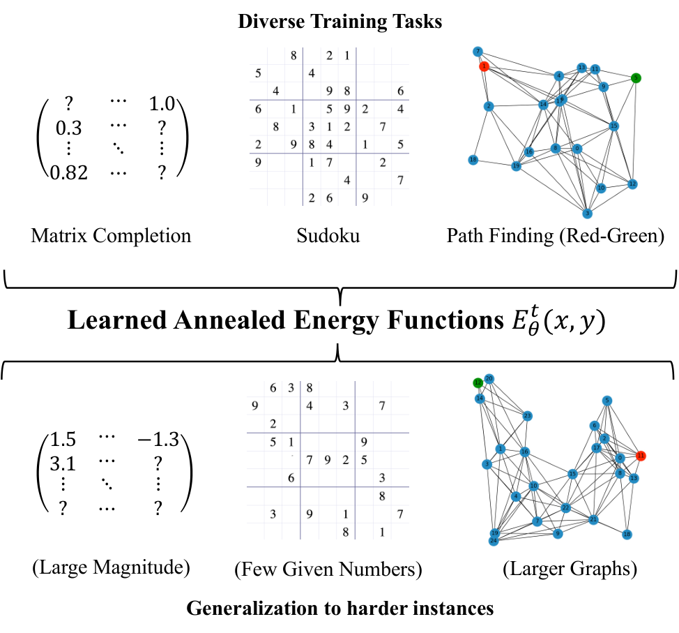
Many reasoning problems can be expressed as selecting an output that satisfies constraints. IRED learns that selection objective from paired inputs and solutions instead of requiring a symbolic task specification. Its central design is an annealed sequence of learned energy landscapes plus training that avoids differentiating through a full optimization rollout. Computation at inference can be increased for difficult instances. The scope is supervised synthetic reasoning tasks; theorem proving and general decision-making motivate the framework but are not demonstrated here.
2 Related Work
Du et al. (2022) previously used iterative energy minimization for learned reasoning. IRED combines that formulation with the noise-conditioned supervision of denoising diffusion models (Ho et al., 2020). It differs from direct diffusion prediction by performing several optimization steps on each landscape rather than relying on one learned reverse transition per stage.
Other approaches insert task-specific solvers or use recurrent computation and learned halting. IRED shares an optimization paradigm across tasks but changes its encoder for matrices, boards, and graphs. Its claimed flexibility therefore does not mean one unchanged network solves every domain.

3 Learning Iterative Reasoning through Energy Optimization
Training learns energies over an input and candidate output. Inference repeatedly refines the output, with the intended energy minimum corresponding to a valid solution. The annealing and contrastive components address difficult optimization and inadequately shaped learned objectives.
3.1 Reasoning as Annealed Energy Minimization
Inference initializes a candidate from Gaussian noise and minimizes its learned energy by gradient descent. Earlier energy-based reasoning trained through the whole optimization trajectory; IRED instead supervises energy gradients at corrupted ground-truth labels. This removes the need to backpropagate through many inference updates during training, though energy-gradient computation itself still requires differentiation. The method’s equations minimize energy; a contrary “maximizes” phrase in the introduction is not the operative objective.
Equations 1–3
| (1) |
| (2) |
| (3) |
3.2 Learning Sequence of Annealed Energy Landscapes
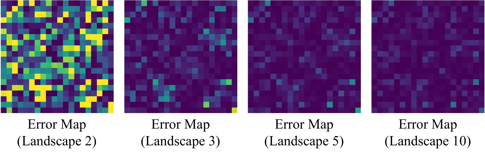
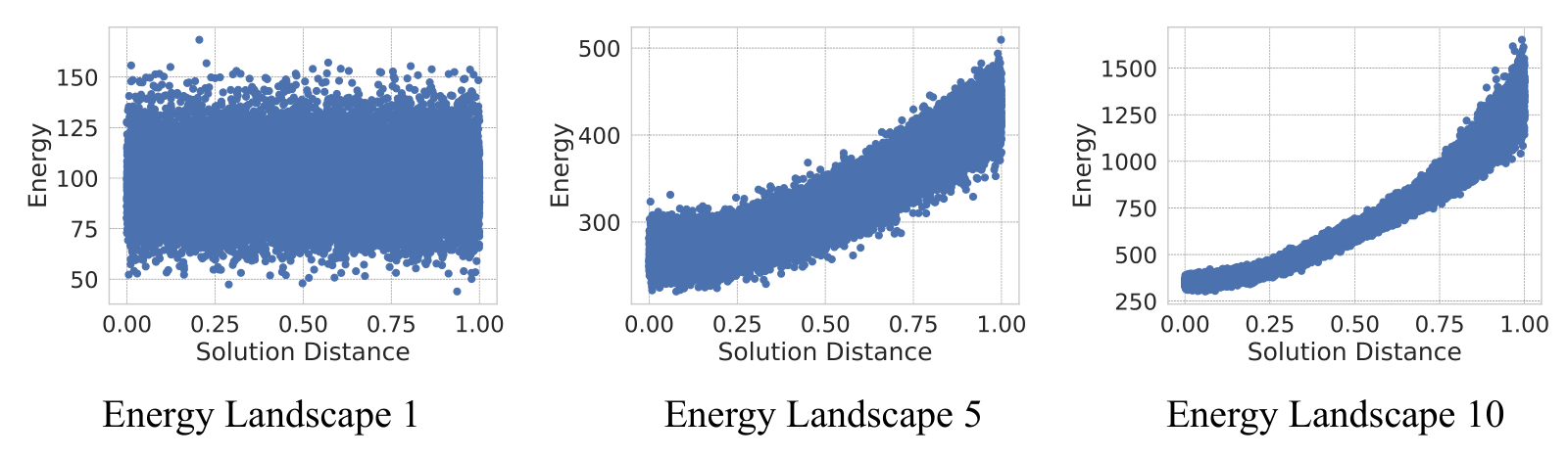
Noise conditioning produces ten landscapes, from smoother high-noise objectives to sharper low-noise ones. At each stage, gradients learn to predict the noise added to a scaled target. Inference optimizes repeatedly at one level, rescales its candidate, and passes it to the next. The schedule eases search empirically, without guaranteeing a convex landscape or global optimum.
Equations 4–5
| (4) |
| (5) |
3.3 Shaping the Energy Landscape
Denoising supervision constrains local gradients but may leave incorrect low-energy solutions elsewhere. A contrastive loss compares a correct label with a corrupted negative under the same sampled noise, favoring the correct candidate. Sharing noise reduces comparison variance. This sampled loss encourages better energy ordering; it cannot enforce global correctness over every possible output.
3.4 Combined Training and Inference Paradigms
The combined objective and complete pseudocode are retained. Training uses a cosine noise schedule and ten landscapes. Inference takes a specified number of gradient steps per landscape and accepts steps that lower energy. The experiments vary that step budget; they do not establish an automatically calibrated stopping rule that detects every wrong solution. Composing extra constraints or representing multiple valid outputs is discussed as a possible extension.
4 Experiments
Evaluation covers matrix operations, symbolic and visual Sudoku, graph connectivity, and graph path decisions. The emphasis is generalization to harder inputs and the effect of additional inference computation.
4.1 Continuous Algorithmic Reasoning
Tasks and comparison. Addition, low-rank completion with half the entries masked, and inversion use 20 × 20 matrices. Harder tests increase value magnitudes or worsen conditioning, rather than increasing matrix dimensions. Models share comparable encoder architectures. Continuous negatives are formed by corrupting labels and taking two energy-optimization steps.
Results. IRED’s harder-test mean squared errors are 0.0020 for addition, 0.2054 for completion, and 0.2063 for inversion, versus IREM’s 0.0021, 0.2074, and 0.2083. The advantages over the previous energy method are modest on these aggregate errors, though larger than several other comparisons. Increasing inversion optimization steps from ten to forty changes harder-test error from 0.2110 to 0.2063; same-distribution error changes from 0.0096 to 0.0095.
Diagnostics. The error maps and energy cross-sections illustrate increasing accuracy and sharper landscapes. Ablations favor gradient optimization, repeated refinement, and contrastive shaping. These visual slices and finite tests do not demonstrate global constraint recovery.
| Same | Harder | ||
|---|---|---|---|
| Task | Method | Difficulty | Difficulty |
| Addition | Feedforward | 0.0448 | 0.7029 |
| Recurrent | 0.3610 | 2.6133 | |
| Programmatic | 0.0111 | 0.3446 | |
| Diffusion | 0.0071 | 0.5931 | |
| IREM | 0.0003 | 0.0021 | |
| IRED (ours) | 0.0002 | 0.0020 | |
| Matrix | Feedforward | 0.0203 | 0.2720 |
| Completion | Recurrent | 0.0266 | 0.3285 |
| Programmatic | 0.0203 | 0.2637 | |
| Diffusion | 0.0219 | 0.2142 | |
| IREM | 0.0183 | 0.2074 | |
| IRED (Ours) | 0.0174 | 0.2054 | |
| Matrix | Feedforward | 0.0112 | 0.2150 |
| Inverse | Recurrent | 0.0109 | 0.2123 |
| Programmatic | 0.0124 | 0.2209 | |
| Diffusion | 0.0115 | 0.2132 | |
| IREM | 0.0108 | 0.2083 | |
| IRED (Ours) | 0.0095 | 0.2063 |
| Opt. Steps | Same Difficulty | Harder Difficulty |
|---|---|---|
| 10 | 0.0096 | 0.2110 |
| 20 | 0.0096 | 0.2100 |
| 30 | 0.0096 | 0.2090 |
| 40 | 0.0095 | 0.2063 |
| Gradient | Optimization | Contrastive | Same | Harder |
|---|---|---|---|---|
| Descent | Refinement | Shaping | Difficulty | Difficulty |
| No | No | No | 0.0158 | 0.2223 |
| Yes | No | No | 0.0097 | 0.2135 |
| Yes | Yes | No | 0.0097 | 0.2113 |
| Yes | Yes | Yes | 0.0095 | 0.2063 |
4.2 Discrete-Space Reasoning
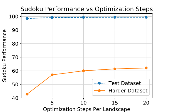
Sudoku and connectivity. Sudoku training uses boards with 31–42 given cells; the harder dataset has 17–34. IRED achieves 99.4% standard-test accuracy and 62.1% on the harder set, compared with RRN’s 99.8% and 28.6%. Thus it leads the harder comparison while the recurrent baseline is slightly better in-distribution. Visual Sudoku replaces symbolic entries with digit images and obtains 98.3%/46.6%. Connectivity grows from at most twelve nodes to eighteen, with accuracy 99.1%/93.8%.
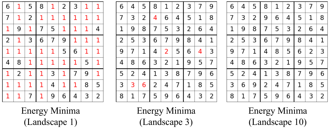
Computation and failure. Additional optimization particularly helps harder Sudoku. The ablation’s harder accuracy rises from 35.0% without the three proposed components to 62.1% with all of them. Nevertheless, the authors observe invalid boards assigned lower energy than the correct solution. More optimization can then prefer the wrong answer, so energy should not be treated as an exact satisfiability test. The full intermediate boards and performance curves are retained.
| Task | Method | Test | Harder |
|---|---|---|---|
| Dataset | Dataset | ||
| Sudoku | IREM | 93.5% | 24.6% |
| Diffusion | 66.1% | 10.3% | |
| SAT-Net | 98.3% | 3.2% | |
| RRN | 99.8% | 28.6% | |
| IRED (ours) | 99.4% | 62.1% | |
| Visual Sudoku | SAT-Net | 63.2% | 0.0% |
| RRN | 99.8% | 28.6% | |
| IRED (ours) | 98.3% | 46.6% | |
| Connectivity | IREM | 94.3% | 89.8% |
| Diffusion | 61.6% | 61.3% | |
| IRED (ours) | 99.1% | 93.8% |
| Gradient | Optimization | Contrastive | Same | Harder |
|---|---|---|---|---|
| Descent | Refinement | Shaping | Difficulty | Difficulty |
| No | No | No | 97.0% | 35.0% |
| Yes | No | No | 98.8% | 45.1% |
| Yes | Yes | No | 99.3% | 59.7% |
| Yes | Yes | Yes | 99.4% | 62.1% |
4.3 Planning
The planner receives a directed graph, start, and goal and predicts a node sequence using a spatial-temporal graph encoder. Training graphs have fifteen nodes and harder tests twenty-five. Evaluation counts whether the first predicted action decreases shortest-path distance; it does not report success for executing the whole generated path or repeated closed-loop episodes.
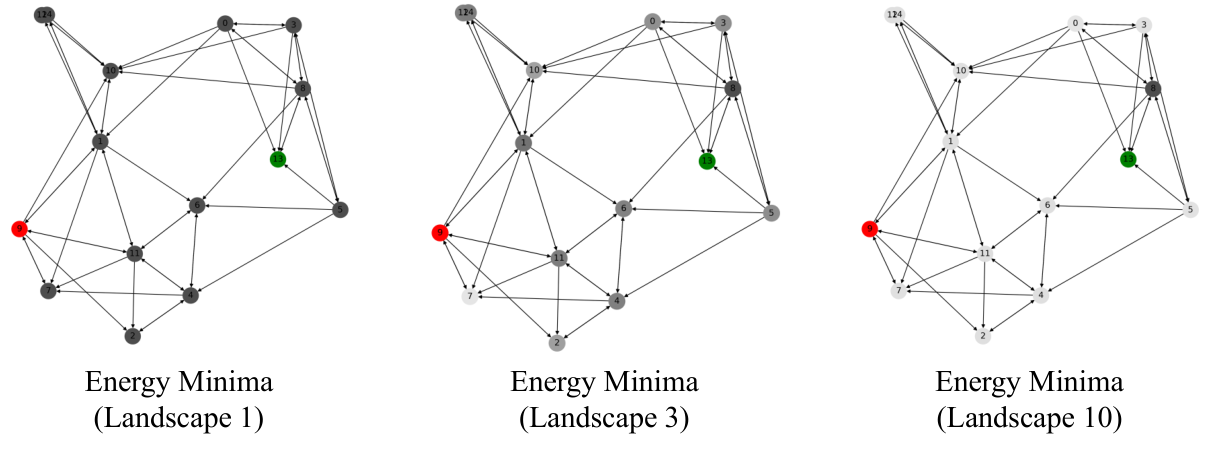
IRED achieves 92.6% and 91.9% first-action success on standard and harder graphs, versus IREM’s 90.4%/88.4% and diffusion’s 45.2%/46.9%. Multi-step optimization and contrastive shaping improve the ablations. Gradient descent alone slightly lowers the first ablated score, so the benefit belongs to the tested combination rather than every component independently improving every task. Figure 7 shows the next-node distribution concentrating during optimization.
| Task | Method | Test | Harder |
|---|---|---|---|
| Dataset | Dataset | ||
| Shortest Path | IREM | 90.4% | 88.4% |
| Diffusion | 45.2% | 46.9% | |
| IRED (ours) | 92.6% | 91.9% |
| Gradient | Optimization | Contrastive | Same | Harder |
|---|---|---|---|---|
| Descent | Refinement | Shaping | Difficulty | Difficulty |
| No | No | No | 80.8% | 80.4% |
| Yes | No | No | 80.7% | 79.1% |
| Yes | Yes | No | 88.6% | 87.9% |
| Yes | Yes | Yes | 92.6% | 91.9% |
5 Conclusion and Discussions
Repeated energy optimization improves selected learned reasoning tasks and permits an inference-compute tradeoff. It still requires many gradient evaluations and is likely slower than specialized solvers when exact task specifications are available. Gaussian annealing is fixed, external intermediate memory is absent, and learned low-energy errors remain possible. Faster initialization, learned schedules, richer memory, hybrid planning, and reward-supervised policies are proposed directions rather than results established by these experiments.
Acknowledgements
Support comes from US research agencies, MIT programs and the MIT–IBM Watson AI Lab, the Simons Center, and a graduate fellowship. The authors state that conclusions are their own.
Impact Statement
The authors identify no immediate negative social impact from the present evaluation on simple standard datasets. Broader deployment effects are not empirically studied in this paper.
Appendix A Experimental Details
Continuous tasks. Models train for about 50,000 iterations with batch size 2,048, Adam at 10⁻⁴, and one RTX 2080, taking roughly two hours. Evaluation uses 20,000 problems. Sudoku uses 50,000 iterations and batch size 64 on the same GPU class.
Graph generation. Nodes are sampled in a unit square and connected to nearby points with randomized out-degree. Connectivity uses degree range 1 to n/2; planning uses 1 to n/5. Edges have unit length, and Floyd–Warshall supplies reachability or shortest-distance targets. Graph models train for 100,000 iterations with batch size 512. These structured graph distributions define the tested generalization setting.
Appendix B Model Architectures
Tables 8–12 preserve complete network layer lists. Continuous energy models use three 512-wide layers and a scalar energy output; the diffusion baseline has an output-sized final layer. Sudoku uses a 384-channel residual convolutional model, with output norm producing energy and direct output producing diffusion noise predictions.
Connectivity and planning use relational architectures based on Neural Logic Machines (Dong et al., 2019). Global pooling creates the scalar energy; diffusion removes that pooling to predict per-edge or per-node noise. Planning additionally stacks adjacent-time embeddings for temporal message passing. These architecture adaptations supply substantial task-appropriate structure while retaining the common training/inference framework.
| Linear 512 |
|---|
| Linear 512 |
| Linear 512 |
| Linear 1 |
| Linear 512 |
|---|
| Linear 512 |
| Linear 512 |
| Linear Output Dim |
| 3x3 Conv2D, 384 |
|---|
| Resblock 384 |
| Resblock 384 |
| Resblock 384 |
| Resblock 384 |
| Resblock 384 |
| Resblock 384 |
| 3x3 Conv2D, 9 |
| NLM Arity=3, Hidden=64 |
|---|
| NLM Arity=3, Hidden=64 |
| Max-Pooling over All Edge Features |
| Linear, 1 |
| NLM Arity=2, Hideen=64 |
|---|
| NLM Arity=2, Hideen=64 |
| Max-Pooling over All Node Features |
| Linear, 1 |