Overview
The complete paper and four supplementary sections are condensed below. All six main figures, four supplementary figures, twelve tables, ten displayed equations, and references are preserved, including every qualitative grid and the explicit occlusion failures.
At a glance
PASTEL combines frozen DINOv2 image features with lightweight semantic and object-boundary heads, then uses multi-scale prediction, heuristic refinement, and recursive normalized cuts to produce panoptic maps. Similarity-selected unlabeled images support one round of semantic self-training. Strong low-label results are reported on driving, general objects, and crop leaves. The direct method is slow—about 200 seconds per image—so the paper also uses it to generate pseudo-labels for a faster segmentation model.
I Introduction
Panoptic segmentation assigns a class to every pixel and distinguishes individual objects. Dense annotation is costly, especially when a robot enters a new domain. PASTEL reduces task-specific labeled-image requirements by relying on a broadly pretrained visual backbone. Its main contribution is the combination of two trainable heads with a boundary-aware fusion procedure and selective self-training. “Few labels” means a small set of fully annotated images, not a small number of annotated pixels or an absence of large-scale pretraining.
II Related Work
Prior methods use sparse points, unlabeled images, pseudo-labels, or broad visual pretraining to reduce supervision. DINOv2 offers descriptive self-supervised features without semantic labels for the target task. PASTEL follows concurrent SPINO in pairing semantic and boundary heads, then adds overlapping multi-scale predictions, cross-class refinement, normalized-cut instance separation, and selected-image self-training. Comparisons mix different backbones, pretraining, and annotation regimes; the tables preserve those distinctions. The paper’s statement about SAM concerns class-agnostic mask generation, rather than a system that directly assigns semantic categories to its masks.
III Technical Approach
The pipeline separates lightweight supervised training from an extensive inference-time fusion process. The latter improves boundaries and class consistency but accounts for substantial computation.
III-A Model Architecture and Training
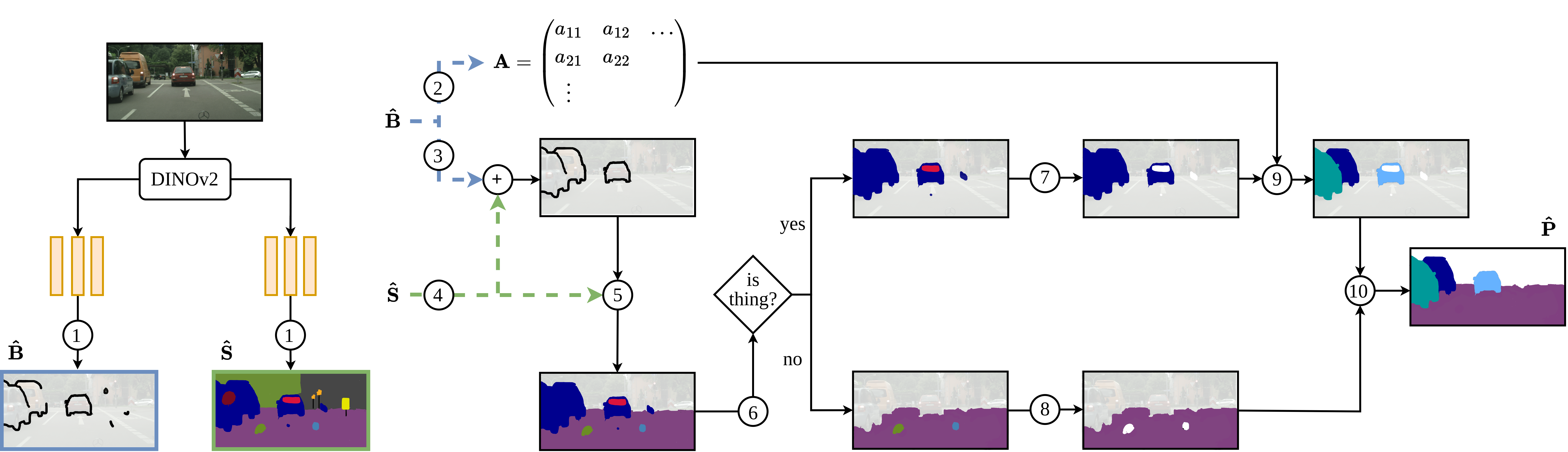
The frozen DINOv2 ViT-B/14 backbone [15] feeds two four-layer 1×1 convolutional heads. Semantic features are upsampled 14× and use channel widths 300, 300, 200, and the class count. Boundary features are upsampled 4× and use widths 600, 600, 400, and one. Semantic training emphasizes uncertain pixels through a bootstrapped cross-entropy threshold of 0.2; boundary training uses binary cross entropy. Heavy crop, resize, flip, and color augmentation expands the small labeled set. Source notation caveat: the prose assigns label zero to boundary pixels and one to background, yet describes the probability as being a boundary; implementation requires a consistent convention. The original equations and descriptions are preserved rather than silently reversing labels.
Equations 1–2
| (1) |
| (2) |
III-B Panoptic Fusion Module
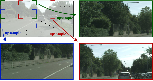
At inference, overlapping crops at several scales are resized to the original image size, processed, downsampled, and averaged. Half-crop overlap avoids seams from disjoint tiling. The fusion module thresholds and denoises predicted boundaries, adds boundaries between semantic regions, and uses majority voting to correct classes within enclosed areas. Connected components identify candidate segments. Small, implausibly enclosed, or boundary-unsupported object regions are temporarily ignored; related filters also apply to background regions. To separate touching instances, a sparse pixel graph assigns lower affinity across stronger boundaries along Bresenham lines. Recursive normalized cuts [29] solve a generalized eigenproblem, using the second-smallest eigenvector, cut-cost and stability thresholds, and a split-point search. This tolerates small gaps that would defeat purely connected-component separation. Tiny results are discarded and nearest-neighbor labels fill ignored pixels. These geometric and size heuristics remain part of the method’s assumptions.
Equations 3–9
| (3) |
| (4) |
| (5) |
| (6) |
| (7) |
| (8) |
| (9) |
III-C Iterative Self-Training
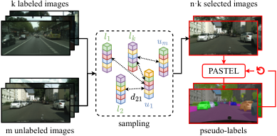
Only the semantic head undergoes self-training because fusion chiefly improves semantic pseudo-label quality. DINOv2 features select the five most similar unlabeled images per labeled example by cosine similarity. PASTEL predicts their pseudo-labels, then trains mixed batches containing one genuine annotation and one pseudo-label. The true-label threshold remains 0.2; pseudo-label loss uses 1.0. Similarity is intended to select examples the current model can label reliably, rather than maximize coverage of unfamiliar scenes.
Equation 10
| (10) |
IV Experimental Evaluation
Experiments evaluate semantic quality with mean intersection-over-union and panoptic quality with a metric combining segmentation and recognition. Results include few-label training, selected unlabeled-image self-training, larger-backbone/label settings, pseudo-label transfer, and component ablations.
IV-A Datasets and Implementation Details
Cityscapes has nineteen driving-scene classes; Pascal VOC has twenty object classes plus background; PhenoBench evaluates crop-leaf instances. Training uses selected images from each training split and evaluates validation data, with an additional PhenoBench test result. Typical experiments use ten labeled Cityscapes images, twenty Pascal VOC images, and fifteen PhenoBench images. Both heads train for 150 epochs on an RTX A6000, taking 11.5 and 16.7 minutes respectively. Direct inference takes about 200 seconds per image, so PASTEL itself is unsuitable for real-time robot perception at these settings.
| Method | Backbone | Supervision | mIoU | PQ | |
| 1a) | Mask2Former [2] | Swin-L | 82.9 | 66.6 | |
| 2a) | PiCIE† [10] | ResNet-18 | 13.8 | – | |
| 2b) | STEGO† [12] | DINO | 38.0 | – | |
| 3a) | ST++ [8] | ResNet-50 | + | 61.4 | – |
| 4a) | ST++ [8] | ResNet-50 | 55.1 | – | |
| 4b) | Hoyer et al. [7] | ResNet-101 | 62.1 | – | |
| 4c) | Hoyer et al.‡ | DINOv2 ViT-B | 46.4 | – | |
| 4d) | ST++‡ | DINOv2 ViT-B | 53.0 | – | |
| 4e) | PanopticDeepLab† [1] | DINOv2 ViT-B | 49.4 | 20.6 | |
| 4f) | Mask2Former‡ | Swin-L | 50.7 | 29.2 | |
| 4g) | SPINO [13] | DINOv2 ViT-B | 61.2 | 36.5 | |
| 5a) | PASTEL (ours) | DINOv2 ViT-L | 75.5 | 50.7 | |
| 5b) | PASTEL (ours) | DINOv2 ViT-S | 64.2 | 41.0 | |
| 5c) | PASTEL (ours) | DINOv2 ViT-B | 63.3 | 41.3 | |
| 5d) | PASTEL (ours) | DINOv2 ViT-B | 64.8 | 42.4 | |
| Method | Backbone | Supervision | mIoU | PQ | |
| 1a) | Panoptic FCN [6] | ResNet-50 | 80.2 | 67.9 | |
| 2a) | MaskContrast [26] | ResNet-50 | 35.0 | – | |
| 2b) | MaskDistill [32] | ResNet-50 | 48.9 | – | |
| 3a) | U2PL [9] | ResNet-101 | + | 68.0 | – |
| 3c) | ST++ [8] | ResNet-50 | + | 65.2 | – |
| 4a) | U2PL [9] | ResNet-101 | 45.8 | – | |
| 4b) | ST++ [8] | ResNet-50 | 50.7 | – | |
| 4c) | ST++‡ | DINOv2 ViT-B | 52.8 | – | |
| 5a) | PASTEL (ours) | DINOv2 ViT-L | 71.1 | 47.3 | |
| 5b) | PASTEL (ours) | DINOv2 ViT-B | 60.6 | 37.0 | |
| 5c) | PASTEL (ours) | DINOv2 ViT-B | 62.5 | 39.5 | |
Supervision methods and denote labeled and unlabeled data, respectively. If a subscript is specified, only images were used for training. ‡: Baseline trained by us.
IV-B Panoptic Segmentation Results
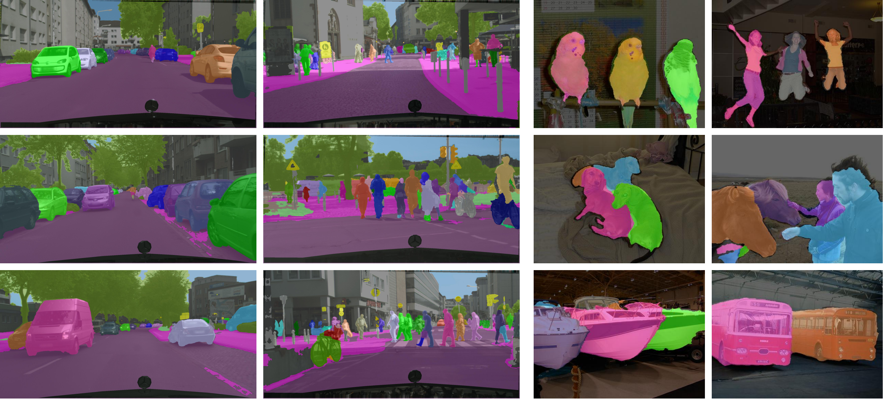
On Cityscapes, ten labels yield 63.3 mIoU and 41.3 PQ, versus SPINO’s 61.2 and 36.5. Adding fifty selected unlabeled images gives 64.8 and 42.4. The strongest displayed PASTEL setting uses a larger ViT-L and 100 annotations, reaching 75.5 mIoU and 50.7 PQ; it is a different budget from the ten-image result. On Pascal VOC, twenty labels give 60.6 mIoU and 37.0 PQ, rising to 62.5 and 39.5 with one hundred pseudo-labeled images. A ViT-L with 92 annotations reaches 71.1 and 47.3. On PhenoBench, fifteen labels produce 51.7 validation PQ and 49.0 test PQ, exceeding Mask R-CNN trained on the same fifteen images but remaining below the fully supervised baseline. Qualitative grids show successful separation alongside pedestrian over-segmentation. For faster deployment, PASTEL trained with ten labels generates pseudo-labels for Mask2Former. Training that model on the Cityscapes training pseudo-labels yields 44.0 PQ; adding the extra split raises it to 44.8, compared with PASTEL’s 42.4. This transfers supervision to an architecture capable of faster inference while still trailing its fully supervised result. The paper refers to Mask2Former’s real-time capability rather than timing the whole pseudo-label pipeline as real-time.

IV-C Ablations and Analysis
The component ablation rises from 30.0 PQ for single-scale connected components to 36.8 with multi-scale prediction, 38.5 with normalized cuts, 41.3 with refinement, and 42.4 after one self-training round. Four participants independently select ten diverse images covering all classes; mean PQ is 40.8±1.4, showing some robustness within this deliberate selection protocol. Increasing labels improves performance, and ViT-L improves over ViT-B; the giant backbone gives only a small PQ increase while slightly lowering mIoU. A second self-training round drops PQ to 41.4 and mIoU to 62.9, consistent with the authors’ overfitting concern. Fifty similarity-selected images give 42.4 PQ versus 38.5±0.5 for fifty random images across three runs. Larger selected sets slightly improve some metrics but do not consistently improve all metrics, so the chosen fifty-image default is a tradeoff.
| Count | mIoU | PQ | SQ | RQ |
| 5 | 57.2 | 36.6 | 69.4 | 46.3 |
| 10 | 63.3 | 41.3 | 74.5 | 52.1 |
| 25 | 67.1 | 43.9 | 75.6 | 55.1 |
| 50 | 69.2 | 46.0 | 76.3 | 57.6 |
| 100 | 70.7 | 47.2 | 76.7 | 59.0 |
| 10 (study) | 64.03.3 | 40.81.4 | 74.31.7 | 51.62.1 |
| DINOv2 | mIoU | PQ | SQ | RQ |
| ViT-S/14 | 53.2 | 34.1 | 73.9 | 42.6 |
| ViT-B/14 | 63.3 | 41.3 | 74.5 | 52.1 |
| ViT-L/14 | 66.2 | 44.2 | 75.0 | 55.9 |
| ViT-g/14 | 65.8 | 44.7 | 75.2 | 56.2 |
| Count | mIoU | PQ | SQ | RQ |
| 0 | 63.7 | 41.4 | 74.9 | 52.1 |
| 10 | 63.5 | 41.5 | 75.1 | 52.1 |
| 50 | 64.8 | 42.4 | 75.7 | 53.1 |
| 100 | 63.7 | 42.6 | 75.3 | 53.4 |
| 200 | 64.8 | 42.5 | 75.3 | 53.4 |
| 50 (random) | 61.81.3 | 38.50.5 | 73.60.3 | 48.50.7 |
We used one iteration of self-training with 50 epochs. For the randomly sampled images, we provide mean and standard deviation over three experiments.
V Conclusion
A strong pretrained representation plus carefully designed fusion can reduce dense target-domain annotation needs. The largest headline gains use larger backbones and annotation budgets than the smallest-label setup. Remaining gaps to full supervision, slow direct inference, occlusion handling, class coverage, and dataset-specific fusion choices constrain the result’s scope.
S-I Pseudo-Labels for Efficient Pretraining
The supplementary experiment uses PASTEL pseudo-labels as pretraining, then fine-tunes Mask2Former on all ground-truth annotations in the Cityscapes training split. It reaches 79.4 mIoU and 63.5 PQ, compared with the cited authors’ fully supervised 77.5 and 62.1. This experiment ultimately uses the full labeled training set, so its gains concern additional pretraining rather than a ten-label-only final system. Its comparison also uses the original authors’ baseline, whereas the main paper reports a somewhat lower local reproduction.
S-II Ablations and Analysis
Reducing resolution to 504×1008 gives 63.5 mIoU and 39.9 PQ, while full 1022×2044 resolution gives 63.3 and 41.3. Quarter-resolution input drops to 56.7 and 31.9, showing the importance of spatial detail for instance quality. Training-epoch results broadly plateau near the 150-epoch default; the authors use a loss-based stopping rule rather than choose the best held-out score from this table. Both supplementary qualitative grids and all boundary overlays are retained.
| Image size | mIoU | PQ | SQ | RQ |
| 56.7 | 31.9 | 71.4 | 41.0 | |
| 63.5 | 39.9 | 73.2 | 50.8 | |
| 63.3 | 41.3 | 74.5 | 52.1 |
| Epoch | mIoU | PQ | SQ | RQ |
| 50 | 60.5 | 39.5 | 74.6 | 49.7 |
| 100 | 63.4 | 41.0 | 74.8 | 51.8 |
| 150 | 63.3 | 41.3 | 74.5 | 52.1 |
| 200 | 63.7 | 41.4 | 74.9 | 52.1 |
| 250 | 63.0 | 41.0 | 75.1 | 51.5 |
S-III Discussion of Limitations
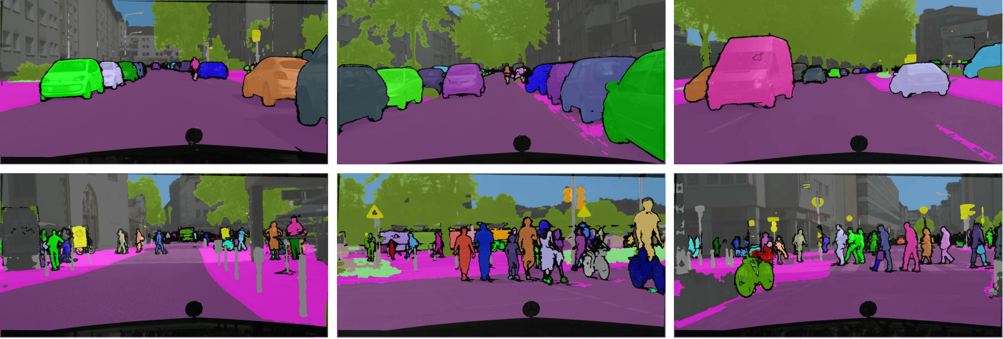
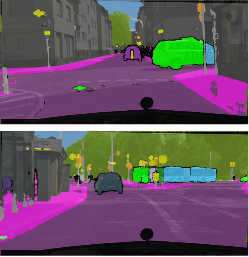
An object split into disconnected visible pieces by occlusion receives multiple instance identifiers: the retained examples show a car split by a traffic light and a bus split by poles. The present two-dimensional boundary mechanism cannot infer their shared hidden extent. Proposed remedies include amodal segmentation or an offset-prediction head, which would need to retain low-label trainability. The small labeled set must also contain every target class; arbitrary random ten-image selection is therefore not the stated protocol.
S-IV Qualitative Results
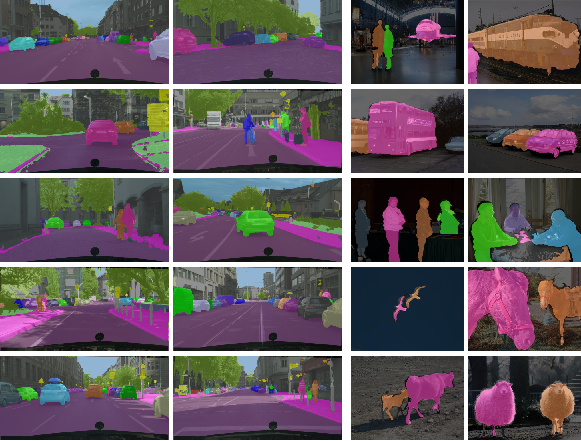
Additional Cityscapes examples span all three validation cities and include distant signs; pedestrian fragments reveal boundary-driven over-segmentation. Pascal VOC examples deliberately emphasize multiple objects rather than its common single-object scenes. PhenoBench grids cover all three growth stages, including increasingly overlapping leaves. These selected examples complement the aggregate metrics and preserve visible successes and failure cases.