At a glance
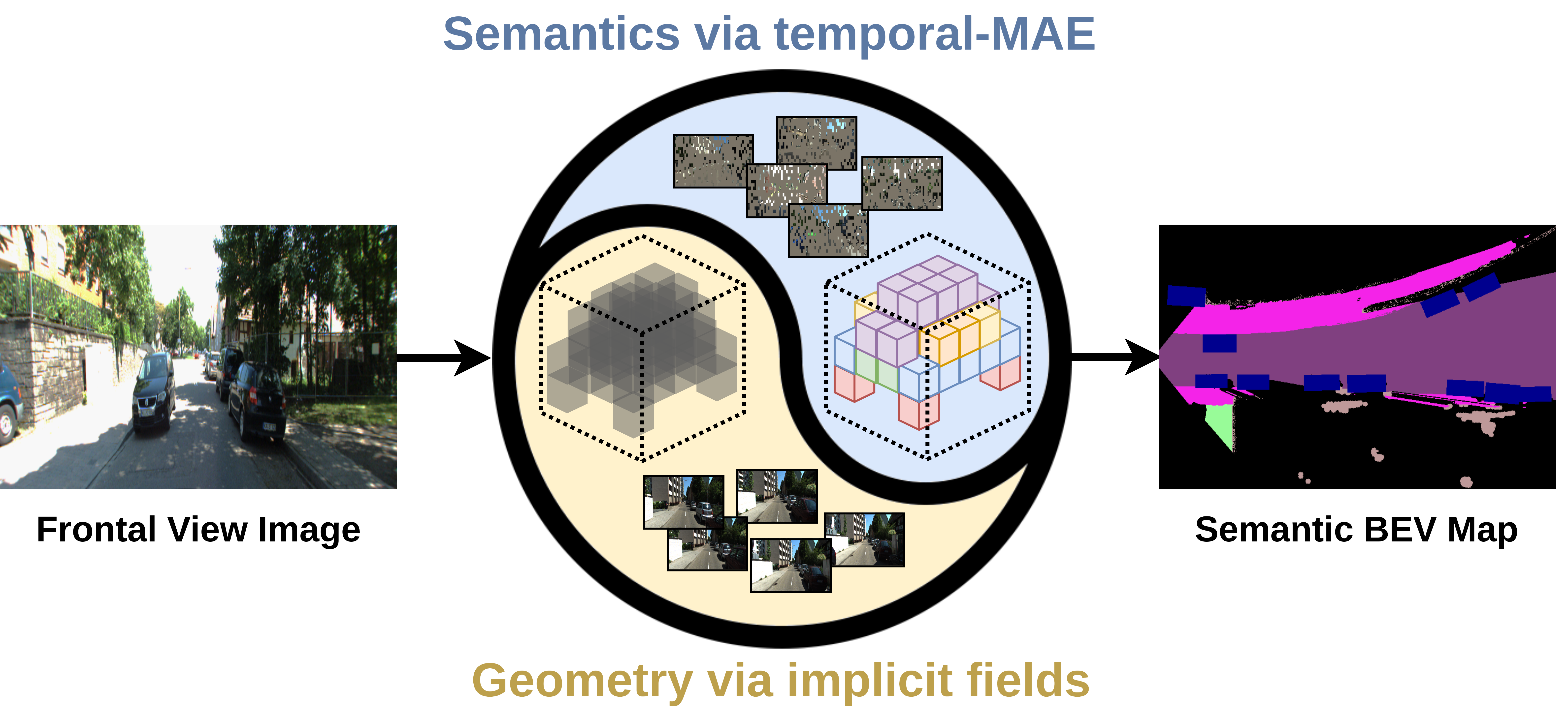
LetsMap predicts a semantic bird’s-eye-view (BEV) map from one frontal image. It first learns scene density and visual representations from unlabeled driving-image sequences through separate geometric and semantic pathways, then learns BEV classes from a small labeled subset. Temporal masked autoencoding reconstructs current and future images from masked current-frame features.
On KITTI-360, the model reaches 28.96% mIoU with 1% BEV labels, versus 30.42% for fully supervised PanopticBEV. It reduces task-specific annotation needs but still uses a pretrained DINOv2 backbone, known camera geometry and motion during pretraining, and labeled BEV data for finetuning. Moving objects remain a major limitation.
1 Introduction
Semantic BEV maps support spatial reasoning beyond the image plane, but dense map annotations are expensive. Prior label-efficient methods either use frontal-view semantic labels or combine labeled and unlabeled BEV data. LetsMap replaces that task-specific semantic pretraining supervision with image consistency and reconstruction.
The contribution is a modular pretraining scheme: one pathway estimates scene geometry, while another learns image features through a temporal masked task. Their features are combined and adapted to BEV segmentation. The final segmentation system is therefore label-efficient rather than entirely unsupervised.
2 Related Work
BEV methods differ in how they lift perspective features into space: learned transformations, explicit geometry, depth distributions, or attention. SkyEye uses frontal semantic supervision; PanopticBEV is a strong fully supervised comparator. LetsMap instead learns image-based pretraining objectives before limited BEV supervision.
The geometry branch draws on image-conditioned neural fields, and the semantic branch extends masked autoencoding across time. A pretrained DINOv2 supplies visual features. The work combines these components for mapping; the external backbone’s prior training remains part of the system.
3 Technical Approach
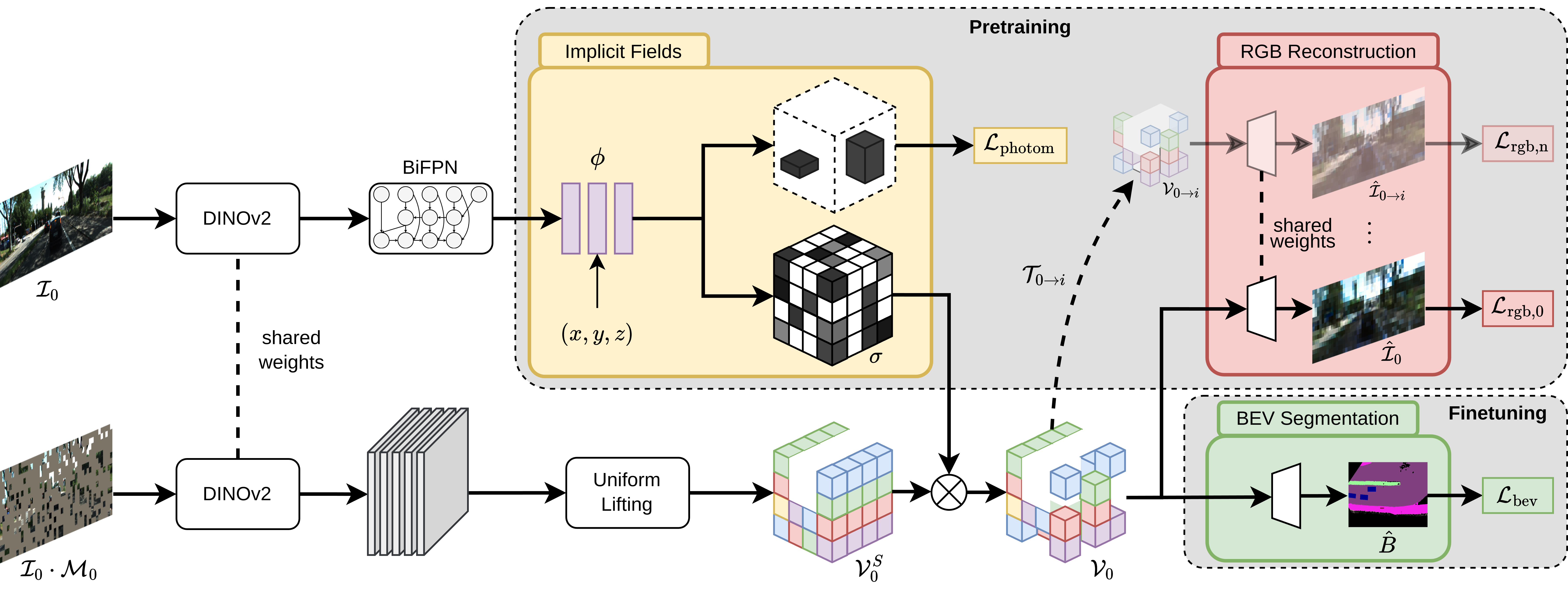
Training has two stages. Frontal-view pretraining combines photometric geometry loss with temporal image-reconstruction loss; BEV finetuning uses semantic cross-entropy. The geometry pathway provides density weights for uniformly lifted semantic features, which are projected differently for the two tasks. Equation 1 retains the stage-dependent objective.
Equation 1
| (1) |
3.1 Network Architecture
A shared pretrained DINOv2 ViT-base backbone supplies three-scale features. The geometry adapter uses a BiFPN and an implicit field; the semantic adapter uses five sparse-convolution layers that propagate the input mask. The supplementary backbone comparison describes the DINOv2 backbone as frozen.
During pretraining, the geometric branch sees the image while the semantic branch sees visible patches of a masked image. Lifted semantic features are multiplied by predicted volumetric density, warped using known camera motion, and projected into current or future frontal views for RGB reconstruction. During finetuning, masking is disabled and features are instead collapsed along height into BEV for semantic prediction.
3.2 Geometric Pathway
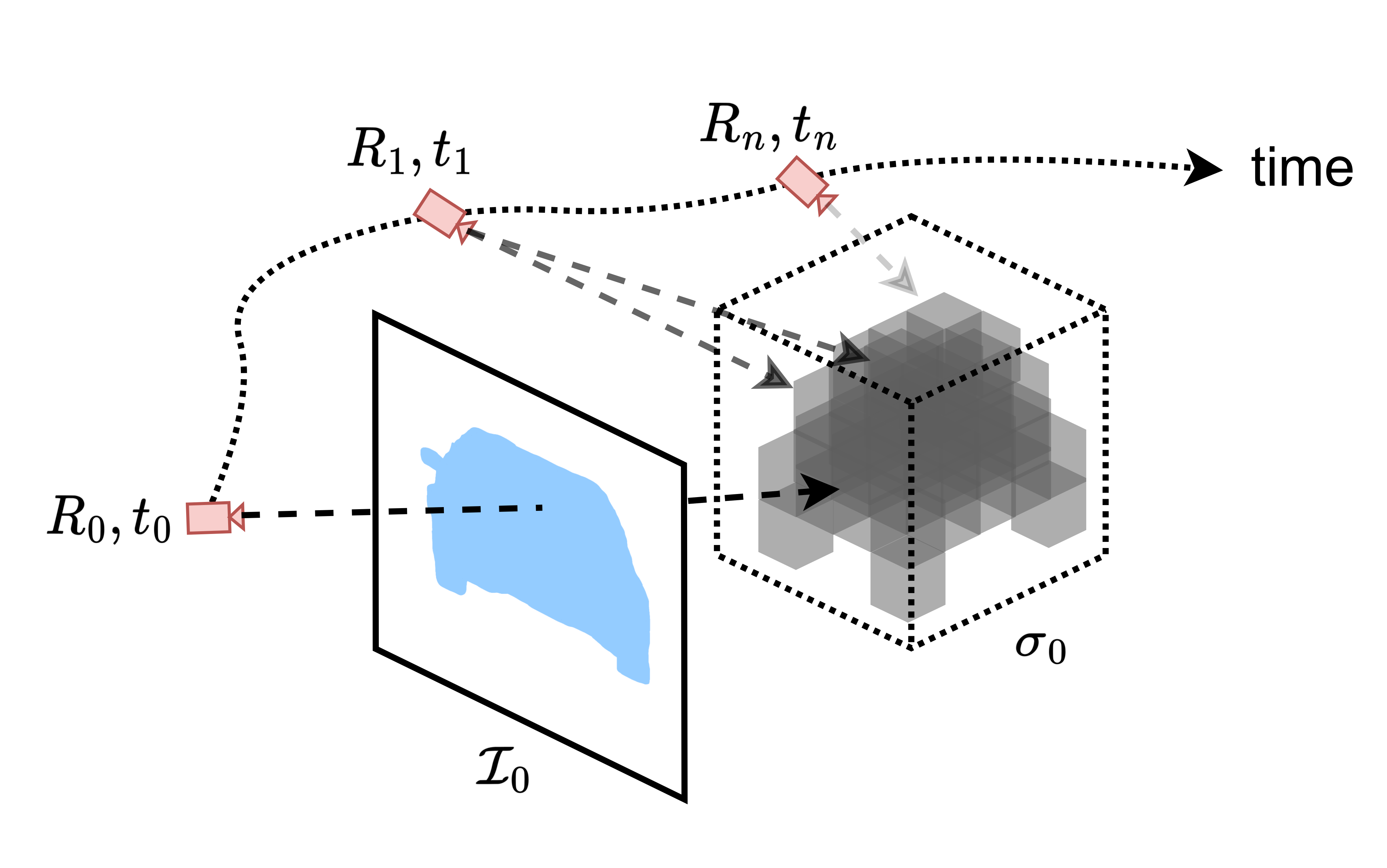
For each sampled 3D point, image features are obtained by projection and bilinear interpolation. A two-layer MLP combines those features with positional encodings of image location and camera distance to predict density. Density along a ray produces an estimated depth, which enables forward and inverse image warping.
Multi-view photometric consistency trains the geometry branch without semantic labels. Pixelwise minima across available views reduce some occlusion effects, but do not eliminate failures from moving objects, limited viewpoints, lighting changes, or inaccurate motion.
The original density, depth, warping, and photometric equations are retained. Equation 3 prints its ray-termination probability as exp(1 − σδ), which can exceed one and is inconsistent with a probability interpretation for some inputs. This source formula is preserved without silently substituting a different expression.
|
|
|
|
Equations 2–7
| (2) |
| (3) | |||
| (4) |
| (5) |
| (6) |
| (7) |
3.3 Semantic Pathway
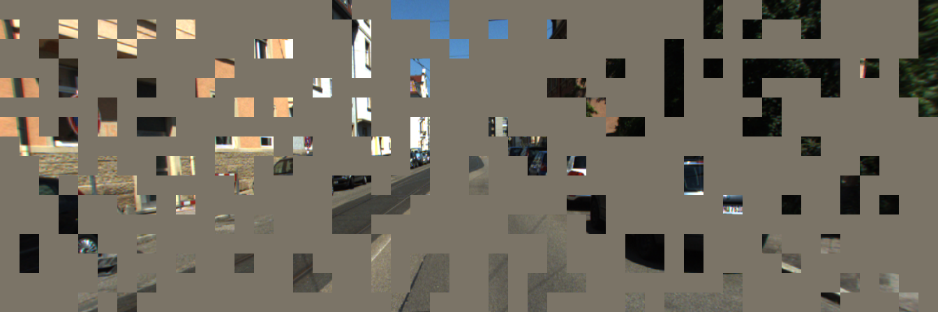
Temporal masked autoencoding (T-MAE) hides patches of the current image and reconstructs both that image and later images. Density-weighted semantic voxels are filled with a shared mask token in missing regions, then warped to other camera poses. An RGB head reconstructs each projected view, supervised by an L2 loss on patch-normalized pixels.
The temporal constraint encourages scene-consistent features. It relies on known camera transforms and works most naturally for static scene elements; an independently moving vehicle does not follow the same warp as the background.
Equations 8–9
| (8) |
| (9) |
3.4 BEV Finetuning
Finetuning removes the RGB reconstruction head, disables masking, and trains semantic BEV predictions with cross-entropy on the available map labels. Monocular inference still uses the learned geometry and representation pathways.
Equation 10
| (10) |
4 Experimental Results
Experiments measure per-class IoU and mean IoU on KITTI-360 and nuScenes, then examine pretraining, backbone size, masking, label budgets, and qualitative map errors.
4.1 Datasets
BEV labels are constructed using the PanopticBEV label-generation pipeline with the occlusion mask discarded. KITTI-360 holds out sequence 10 and uses the other eight sequences for training. nuScenes uses the cited split of 702 training and 142 validation sequences.
KITTI-360 pretraining obtains additional forward-facing perspective views from fisheye cameras. nuScenes training uses one camera because the authors consider overlap between its spatial cameras insufficient. Thus the multi-camera supervision available to the geometry branch differs between datasets.
4.2 Training Protocol
Input sizes are 448×1344 for KITTI-360 and 448×896 for nuScenes. Pretraining uses a four-frame window, 75% masking, 28-pixel patches, and twenty epochs. SGD uses batch size 12, momentum 0.9, weight decay 10⁻⁴, and initial learning rate 0.005, reduced at epochs 15 and 18.
The main finetuning protocol specifies 100 epochs with the same starting learning rate, reduced at epochs 75 and 90. KITTI-360 uses 1% BEV labels; nuScenes selects one labeled sample per training scene. The source writes that latter budget as approximately 1/40% in several places but also calls it 1% elsewhere, so the unambiguous sampling rule is reported here. Table 3’s label-budget experiments additionally use different epoch counts across splits.
4.3 Quantitative Results
With 1% KITTI-360 BEV labels, LetsMap scores 28.96% mIoU, exceeding SkyEye’s 26.94% under the same BEV budget even though SkyEye also uses full frontal-view labels. It exceeds four older fully supervised baselines but remains below fully supervised PanopticBEV at 30.42%. At the same 1% budget, PanopticBEV reaches 19.09%.
On nuScenes, LetsMap reaches 27.66% mIoU with the one-sample-per-scene protocol, compared with 24.03% for PanopticBEV under that small budget and 30.90% for fully supervised PanopticBEV. Fully supervised PON also scores higher at 28.09%. SkyEye is not evaluated there because the required frontal semantic labels are unavailable.
Dynamic classes expose the geometry limitation. Relative to fully supervised PanopticBEV, LetsMap is lower by 8.83 and 3.80 points on KITTI-360 car and truck IoU, and by 9.68 and 7.70 points on nuScenes. The evidence supports reduced annotation cost with a remaining accuracy gap, not universal equality with the best fully supervised model.
| Method | FV | BEV | Road | Side. | Build. | Terrain | Person | 2-Wh. | Car | Truck | mIoU |
| IPM [24] | 100% | - | 53.03 | 24.90 | 15.19 | 32.31 | 0.20 | 0.36 | 11.59 | 1.90 | 17.44 |
| VED [23] | - | 100% | 65.97 | 35.41 | 37.28 | 34.34 | 0.13 | 0.07 | 23.83 | 8.89 | 25.74 |
| VPN [28] | - | 100% | 69.90 | 34.31 | 33.65 | 40.17 | 0.56 | 2.26 | 27.76 | 6.10 | 26.84 |
| PON [30] | - | 100% | 67.98 | 31.13 | 29.81 | 34.28 | 2.28 | 2.16 | 37.99 | 8.10 | 26.72 |
| PoBEV [10] | - | 100% | 70.14 | 35.23 | 34.68 | 40.72 | 2.85 | 5.63 | 39.77 | 14.38 | 30.42 |
| PoBEV [10] | - | 1% | 60.41 | 20.97 | 24.65 | 23.38 | 0.15 | 0.23 | 21.71 | 1.23 | 19.09 |
| SkyEye [9] | 100% | 1% | 69.26 | 33.48 | 32.79 | 39.46 | 0.00 | 0.34 | 32.36 | 7.93 | 26.94 |
| LetsMap (Ours) | 0% | 1% | 70.58 | 34.26 | 40.68 | 38.53 | 1.35 | 4.74 | 30.94 | 10.58 | 28.96 |
| Method | FV | BEV | Road | Side. | Manm. | Terrain | Person | 2-Wh. | Car | Truck | mIoU |
| IPM [24] | 100% | - | 43.51 | 9.05 | 26.21 | 16.60 | 0.14 | 0.72 | 4.65 | 3.67 | 13.07 |
| VED [23] | - | 100% | 67.97 | 25.23 | 49.69 | 31.51 | 0.80 | 1.28 | 21.85 | 17.51 | 26.98 |
| VPN [28] | - | 100% | 66.47 | 23.94 | 47.65 | 33.19 | 2.02 | 4.13 | 22.66 | 18.33 | 27.30 |
| PON [30] | - | 100% | 67.50 | 24.49 | 47.02 | 30.86 | 2.49 | 6.85 | 26.68 | 18.85 | 28.09 |
| PoBEV [10] | - | 100% | 70.15 | 27.87 | 50.04 | 35.32 | 3.89 | 7.06 | 31.60 | 21.27 | 30.90 |
| PoBEV [10] | - | 64.55 | 19.85 | 45.21 | 28.45 | 1.20 | 1.06 | 20.45 | 11.48 | 24.03 | |
| LetsMap (Ours) | 0% | 67.72 | 27.06 | 47.10 | 34.78 | 3.31 | 5.79 | 21.92 | 13.57 | 27.66 |
4.4 Ablation Study
The label-budget study samples three random labeled subsets at each of 1%, 5%, 10%, 50%, and 100% and reports mean performance. LetsMap’s task-specific pretraining improves its no-pretraining counterpart most at 1%: 28.96 versus 26.47 mIoU. The 5% result, 31.90, exceeds the original PanopticBEV backbone trained on all labels at 30.42.
More labels do not produce strictly increasing LetsMap scores in Table 3: 1%, 5%, 10%, 50%, and 100% give 28.96, 31.90, 33.33, 32.54, and 32.88. Epoch counts vary across those settings. SkyEye exceeds LetsMap’s aggregate result at the two largest budgets and often performs better on person, two-wheeler, and car classes.
At 1% labels, geometry pretraining increases mIoU from 26.47 to 27.75, and adding T-MAE raises it to 28.96. Masking ratios of 0%, 25%, 50%, 75%, and 90% yield 27.75, 27.87, 28.22, 28.96, and 27.31. The selected 75% ratio is best among these tested settings; the proposed difficulty-versus-information explanation is an interpretation of the ablation.
| BEV | Model | FV | PT | Epochs | Road | Side | Build | Terr. | Pers. | 2-Wh. | Car | Truck | mIoU |
|---|---|---|---|---|---|---|---|---|---|---|---|---|---|
| 1% | PoBEV | ✗ | - | 100 | 60.41 | 20.97 | 24.65 | 23.38 | 0.15 | 0.23 | 21.71 | 1.23 | 19.09 |
| SkyEye | ✓ | ✓ | 69.26 | 33.48 | 32.79 | 39.46 | 0.00 | 0.34 | 32.36 | 7.93 | 26.94 | ||
| LetsMap | ✗ | ✗ | 69.40 | 32.09 | 34.75 | 35.27 | 1.01 | 2.79 | 28.76 | 7.66 | 26.47 | ||
| LetsMap | ✗ | ✓ | 70.58 | 34.26 | 40.68 | 38.53 | 1.35 | 4.74 | 30.94 | 10.58 | 28.96 | ||
| 5% | PoBEV | ✗ | - | 80 | 64.45 | 27.36 | 30.15 | 31.66 | 0.69 | 0.98 | 29.75 | 6.06 | 23.89 |
| SkyEye | ✓ | ✓ | 72.16 | 37.20 | 34.89 | 42.97 | 4.77 | 9.16 | 40.74 | 9.88 | 31.47 | ||
| LetsMap | ✗ | ✗ | 72.80 | 37.89 | 38.59 | 40.06 | 2.34 | 5.62 | 34.86 | 16.26 | 31.05 | ||
| LetsMap | ✗ | ✓ | 73.74 | 39.56 | 42.07 | 41.49 | 2.46 | 6.32 | 34.68 | 14.88 | 31.90 | ||
| 10% | PoBEV | ✗ | - | 50 | 66.58 | 30.28 | 31.76 | 34.50 | 1.22 | 3.28 | 33.43 | 7.56 | 26.08 |
| SkyEye | ✓ | ✓ | 73.36 | 38.30 | 37.54 | 44.62 | 4.80 | 9.67 | 42.84 | 10.06 | 32.65 | ||
| LetsMap | ✗ | ✗ | 74.31 | 38.45 | 40.04 | 41.26 | 3.19 | 6.02 | 35.56 | 16.53 | 31.92 | ||
| LetsMap | ✗ | ✓ | 74.74 | 39.40 | 43.63 | 43.33 | 2.91 | 6.95 | 37.62 | 18.09 | 33.33 | ||
| 50% | PoBEV | ✗ | - | 30 | 69.88 | 33.81 | 33.40 | 40.48 | 2.47 | 4.63 | 38.81 | 9.84 | 29.16 |
| SkyEye | ✓ | ✓ | 73.10 | 39.23 | 38.08 | 45.72 | 4.05 | 10.44 | 44.72 | 12.10 | 33.43 | ||
| LetsMap | ✗ | ✗ | 73.89 | 38.42 | 42.25 | 41.46 | 2.26 | 6.26 | 37.20 | 15.08 | 32.10 | ||
| LetsMap | ✗ | ✓ | 74.29 | 38.48 | 43.87 | 42.77 | 2.80 | 5.22 | 37.68 | 15.20 | 32.54 | ||
| 100% | PoBEV | ✗ | - | 20 | 70.14 | 35.23 | 34.68 | 40.72 | 2.85 | 5.63 | 39.77 | 14.38 | 30.42 |
| SkyEye | ✓ | ✓ | 73.57 | 39.45 | 38.74 | 46.06 | 3.95 | 9.66 | 45.21 | 10.92 | 33.44 | ||
| LetsMap | ✗ | ✗ | 74.22 | 39.39 | 42.86 | 42.96 | 2.55 | 6.66 | 35.68 | 17.11 | 32.68 | ||
| LetsMap | ✗ | ✓ | 74.81 | 38.59 | 42.58 | 43.67 | 3.52 | 6.21 | 38.47 | 15.24 | 32.88 |
| Model | Geometric | Semantic | Road | Side. | Build. | Terr. | Pers. | 2-Wh. | Car | Truck | mIoU |
|---|---|---|---|---|---|---|---|---|---|---|---|
| L1 | ✗ | ✗ | 69.40 | 32.09 | 34.75 | 35.27 | 1.01 | 2.79 | 28.76 | 7.66 | 26.47 |
| L2 | ✓ | ✗ | 70.85 | 34.34 | 38.12 | 35.03 | 0.93 | 4.06 | 29.79 | 8.84 | 27.75 |
| L3 | ✓ | ✓ | 70.58 | 34.26 | 40.68 | 38.53 | 1.35 | 4.74 | 30.94 | 10.58 | 28.96 |
| Masking Ratio | 0% | 25% | 50% | 75% | 90% |
|---|---|---|---|---|---|
| mIoU | 27.75 | 27.87 | 28.22 | 28.96 | 27.31 |
| Input FV Image | SkyEye/PoBEV | LetsMap (Ours) | Improvement/Error | |
|
(a) KITTI-360 |
|
|
|
|
|
(b) KITTI-360 |
|
|
|
|
|
(c) KITTI-360 |
|
|
|
|
|
(d) nuScenes |
|
|
|
|
|
(e) nuScenes |
|
|
|
|
|
(f) nuScenes |
|
|
|
|
4.5 Qualitative Results
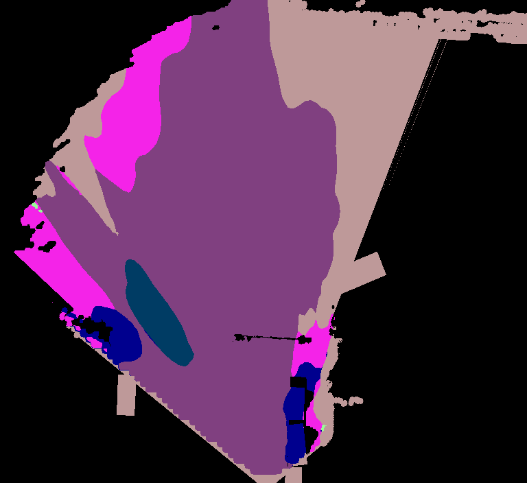
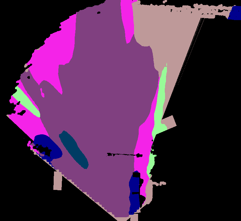
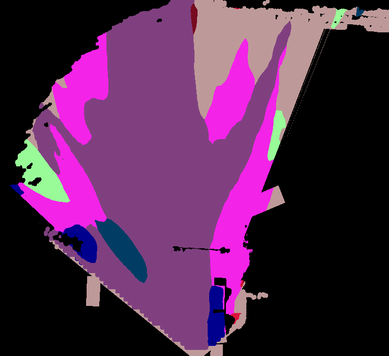
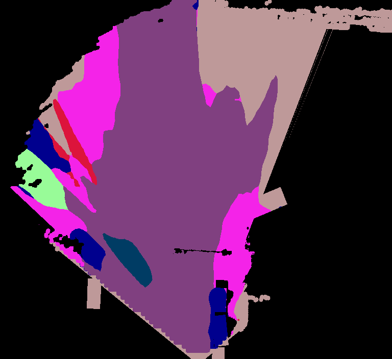
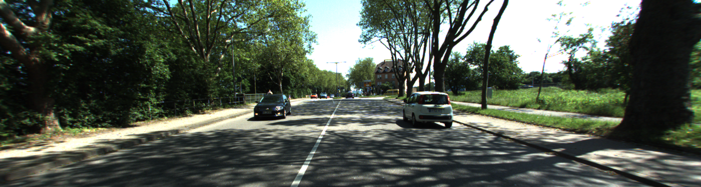
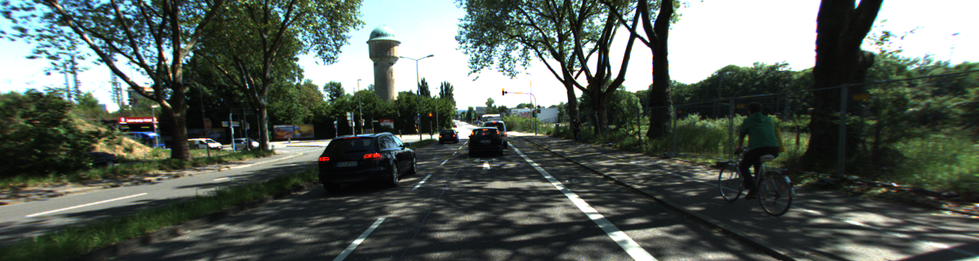
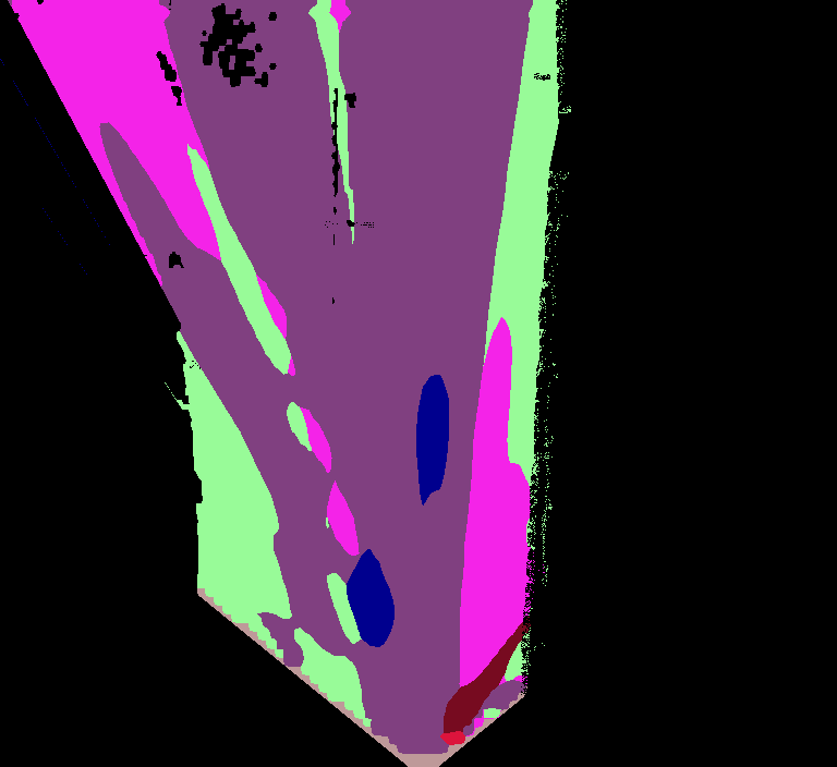
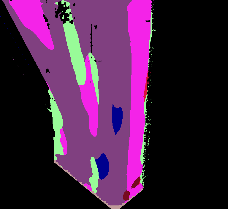
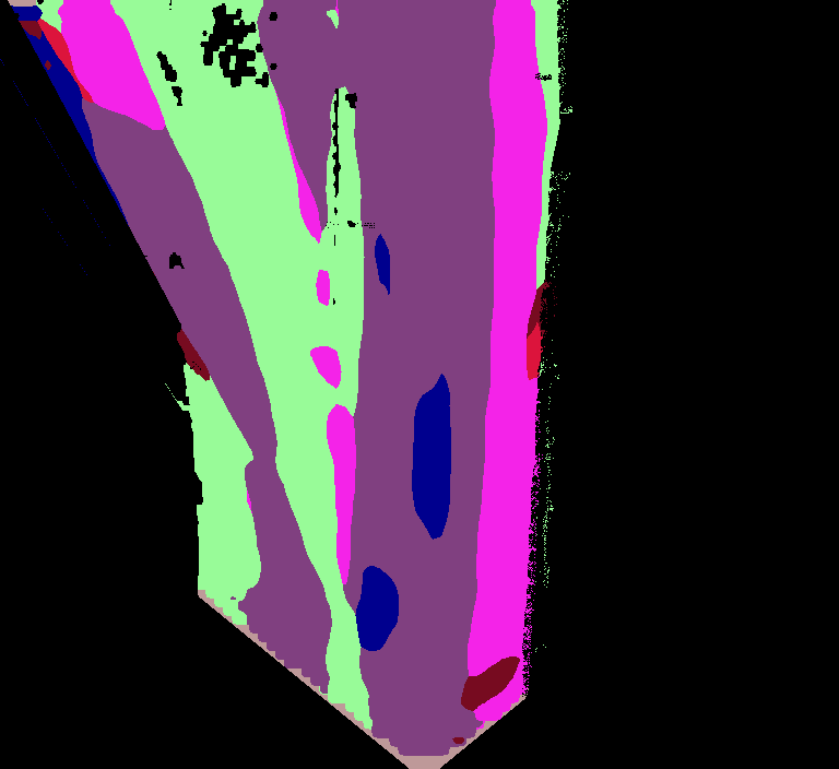
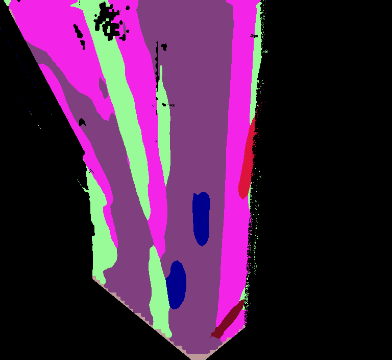
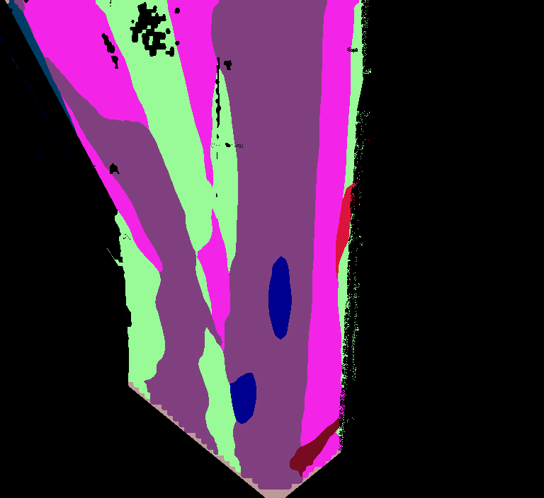
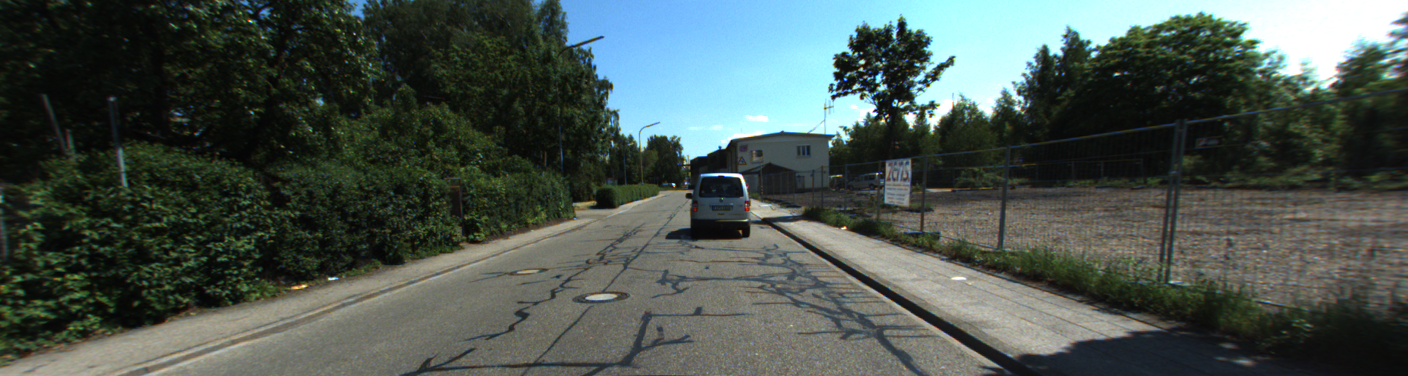
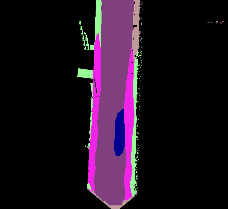
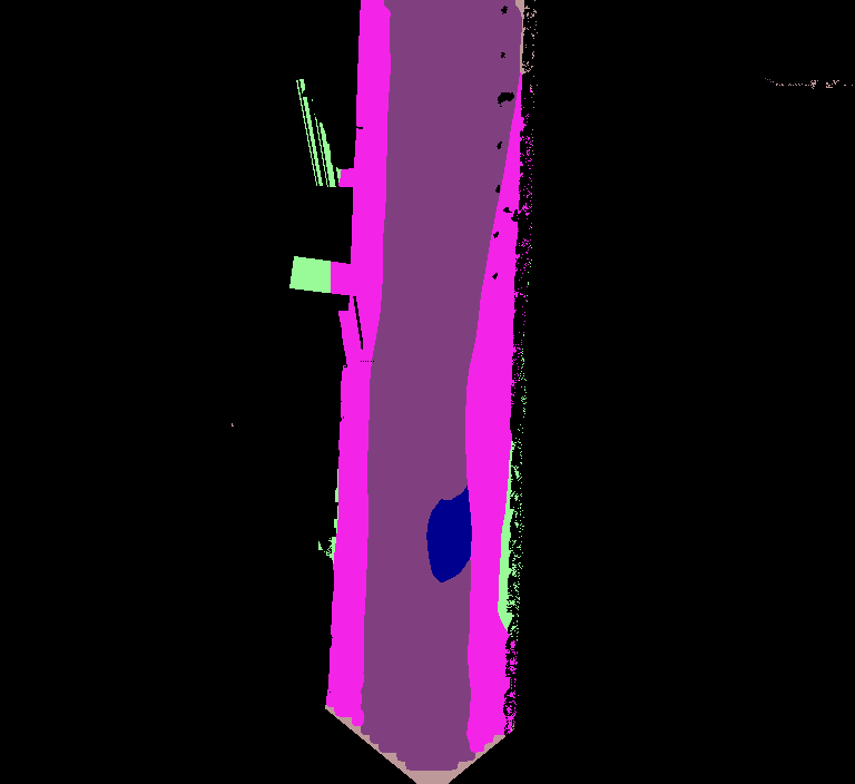
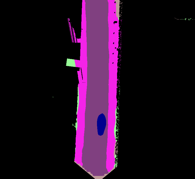
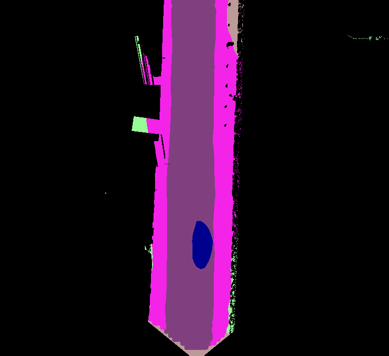
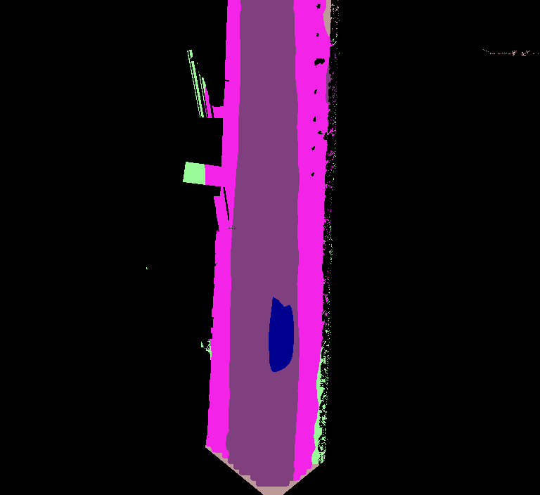
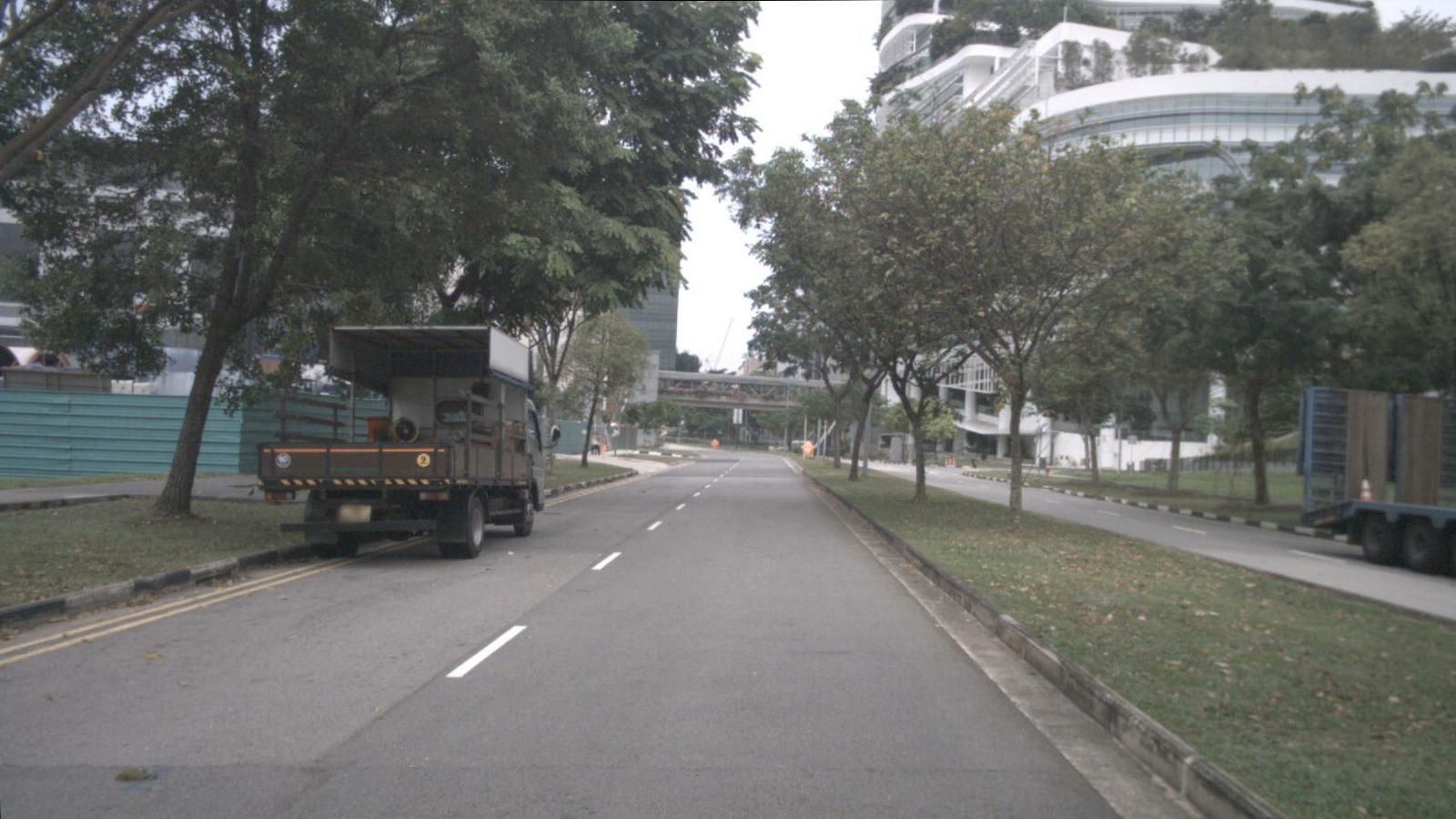
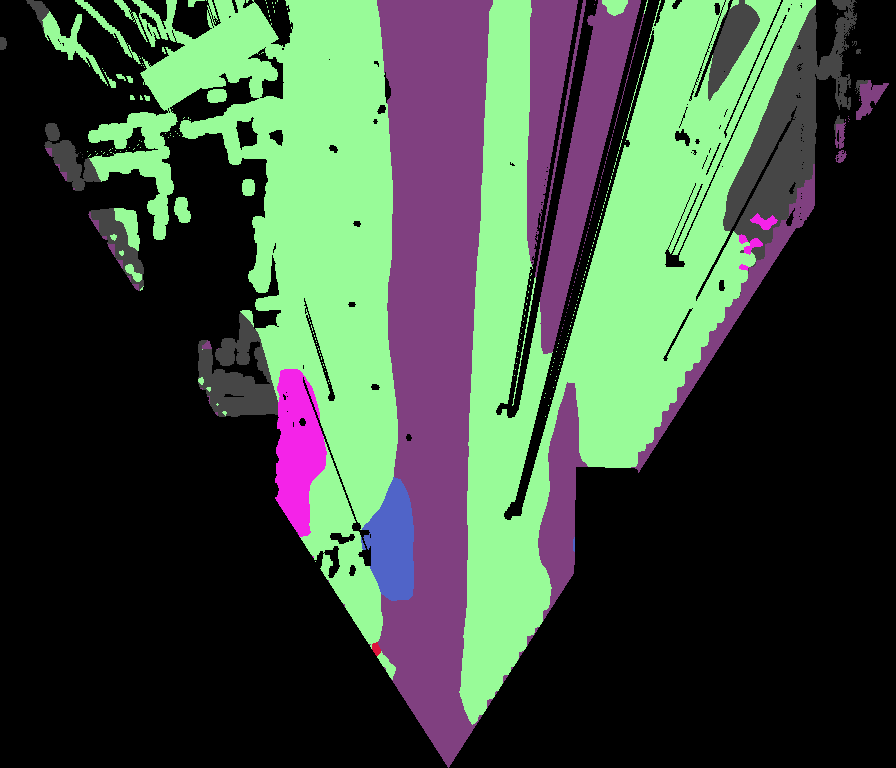
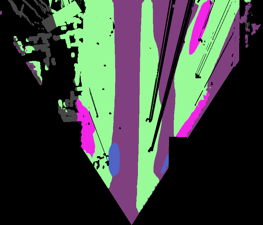
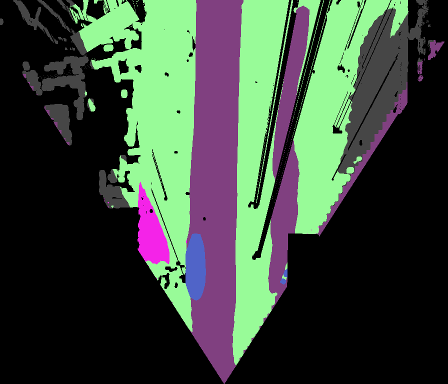
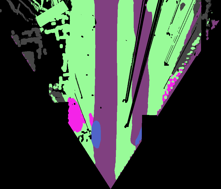
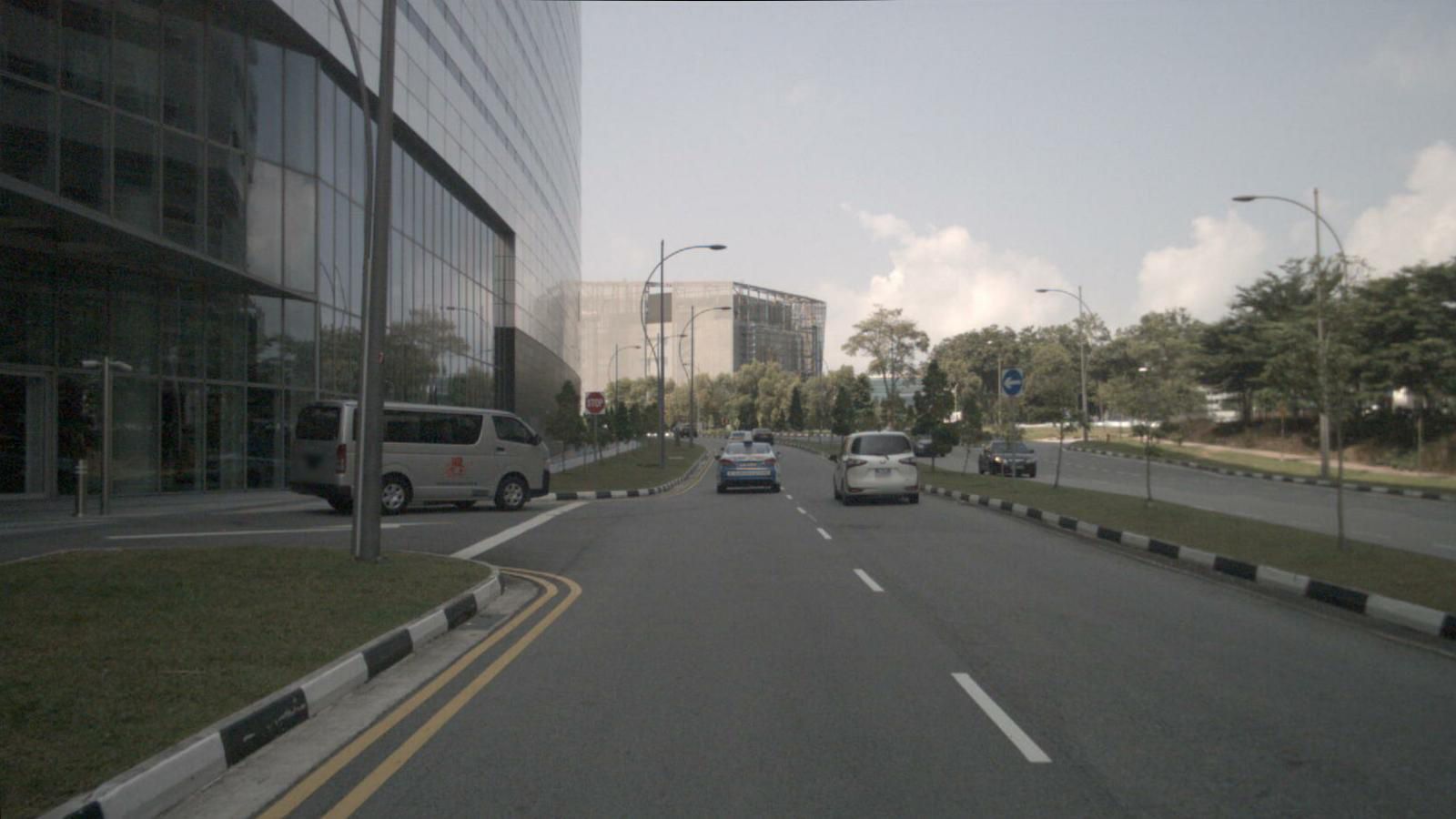
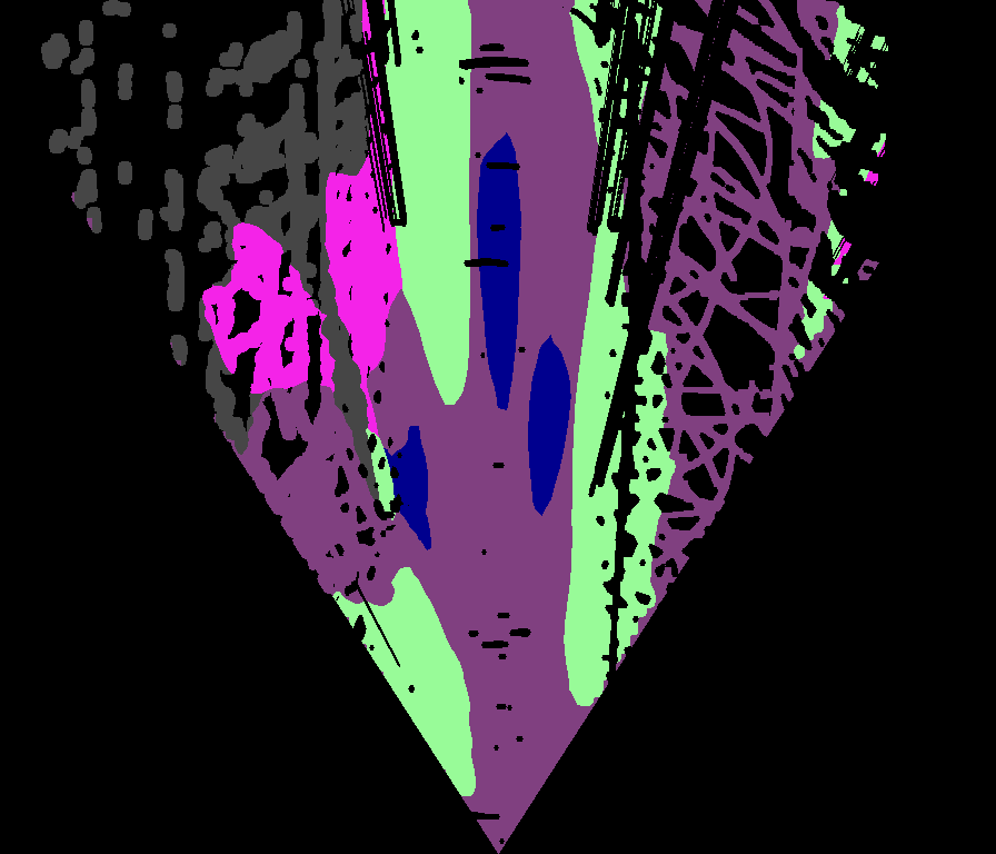
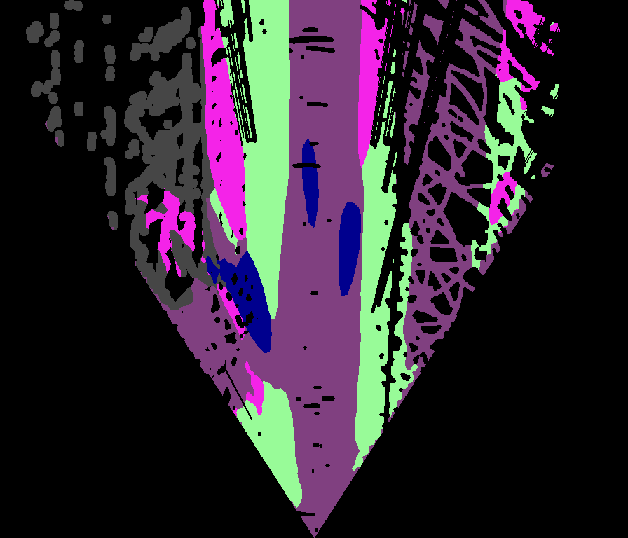
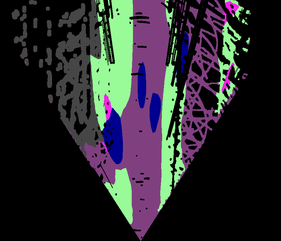
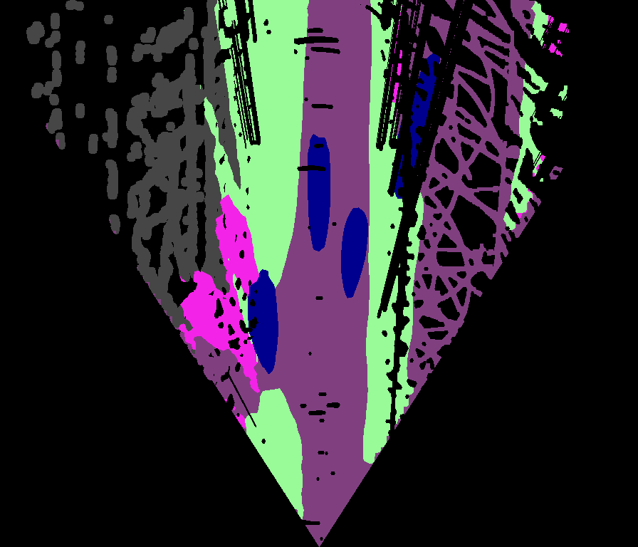
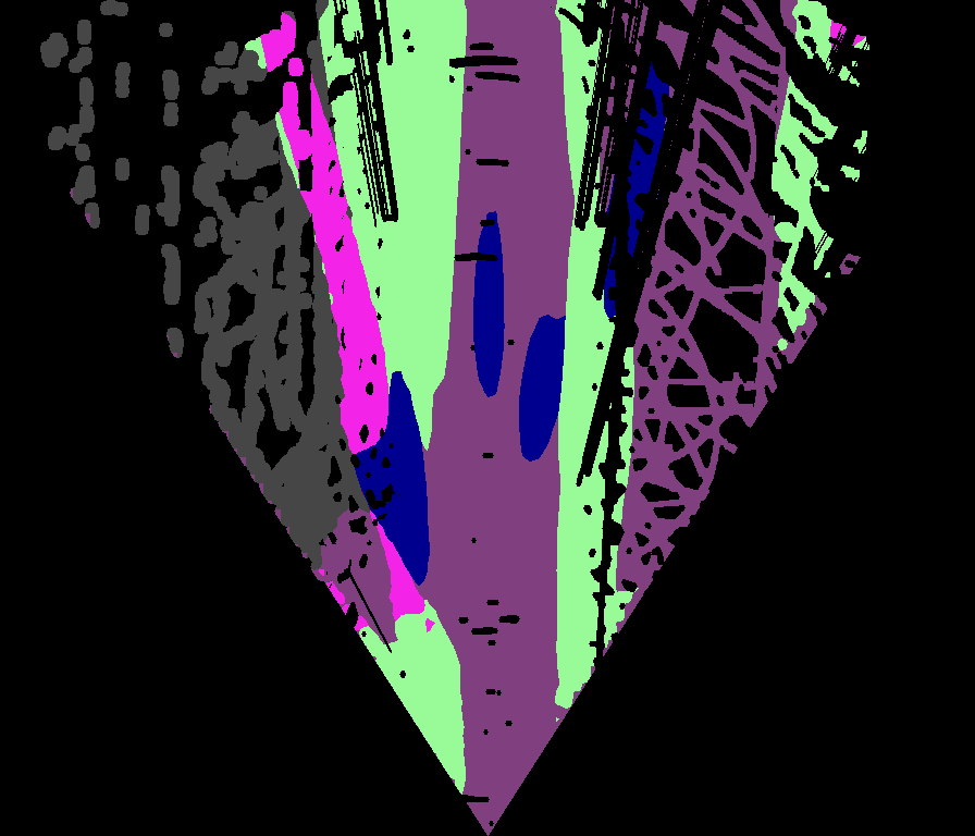
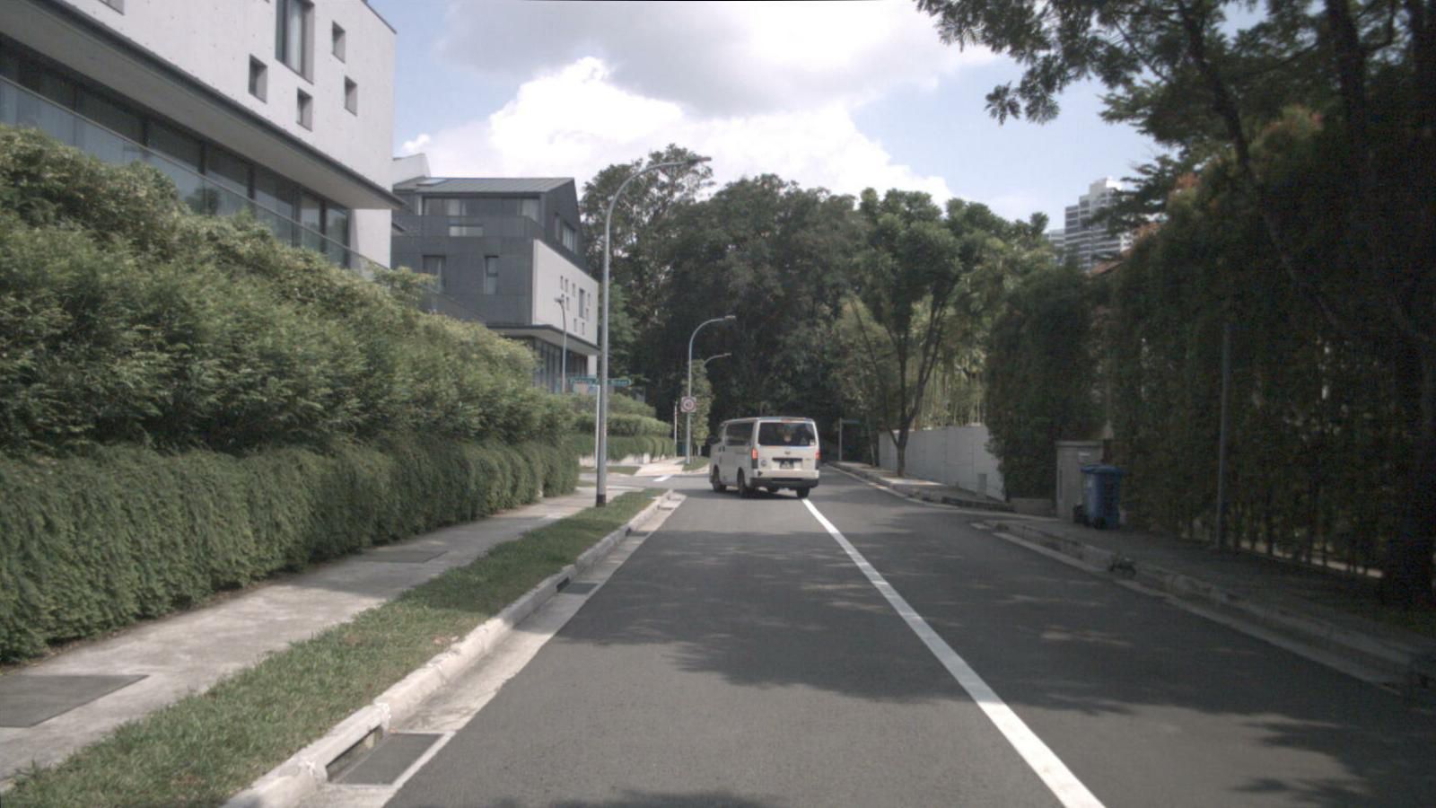
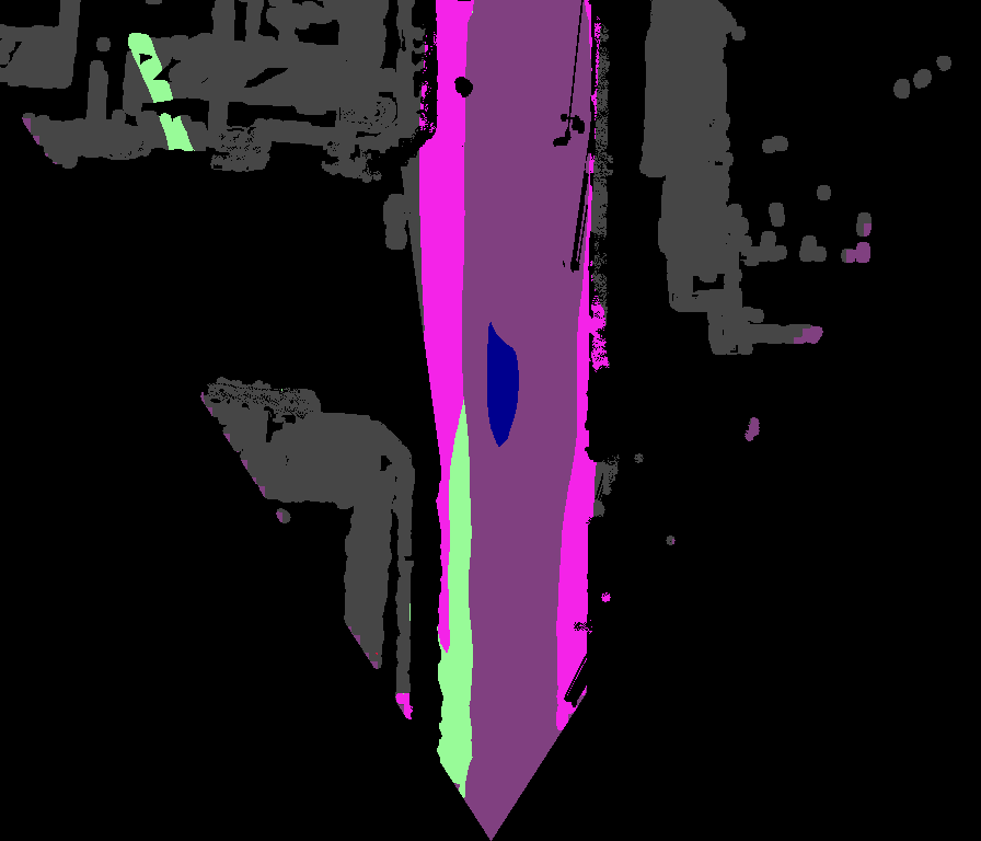
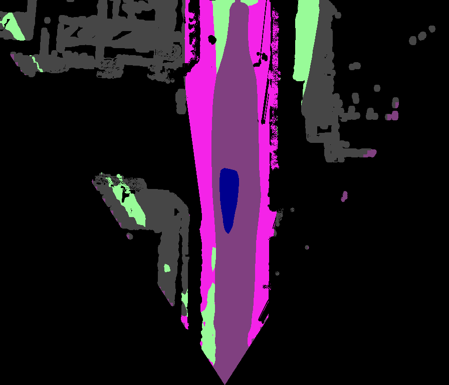
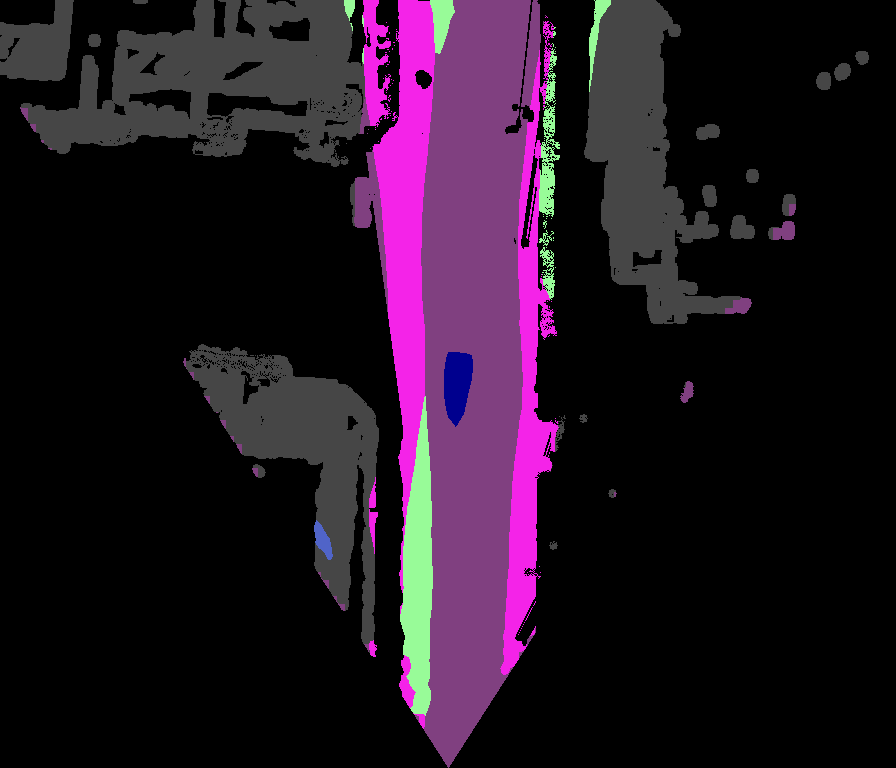
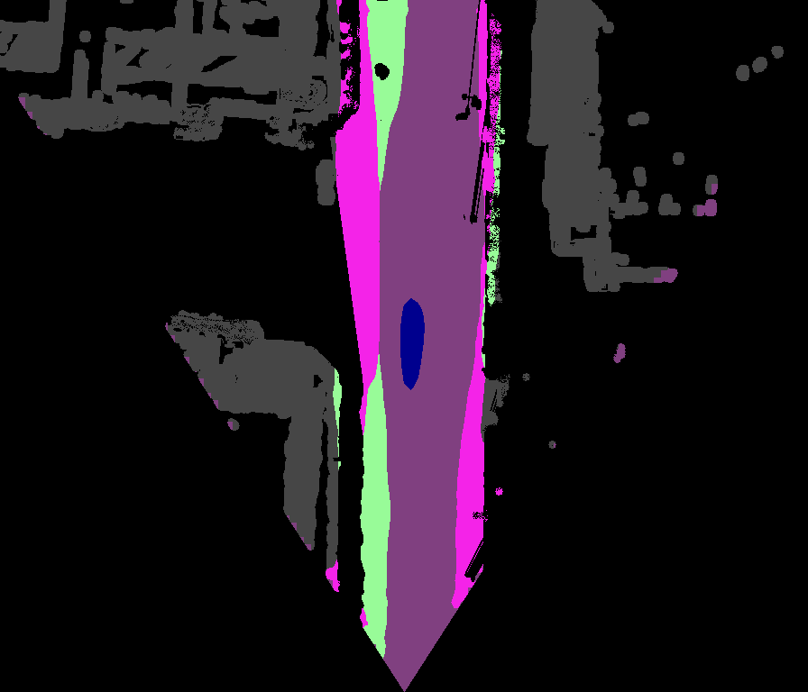
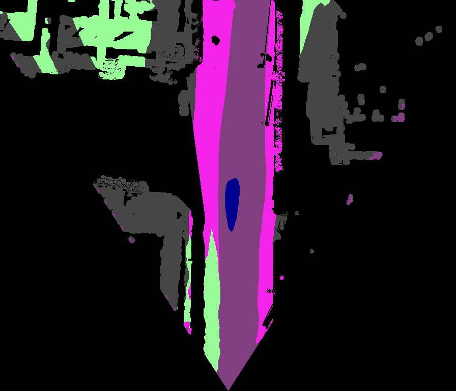
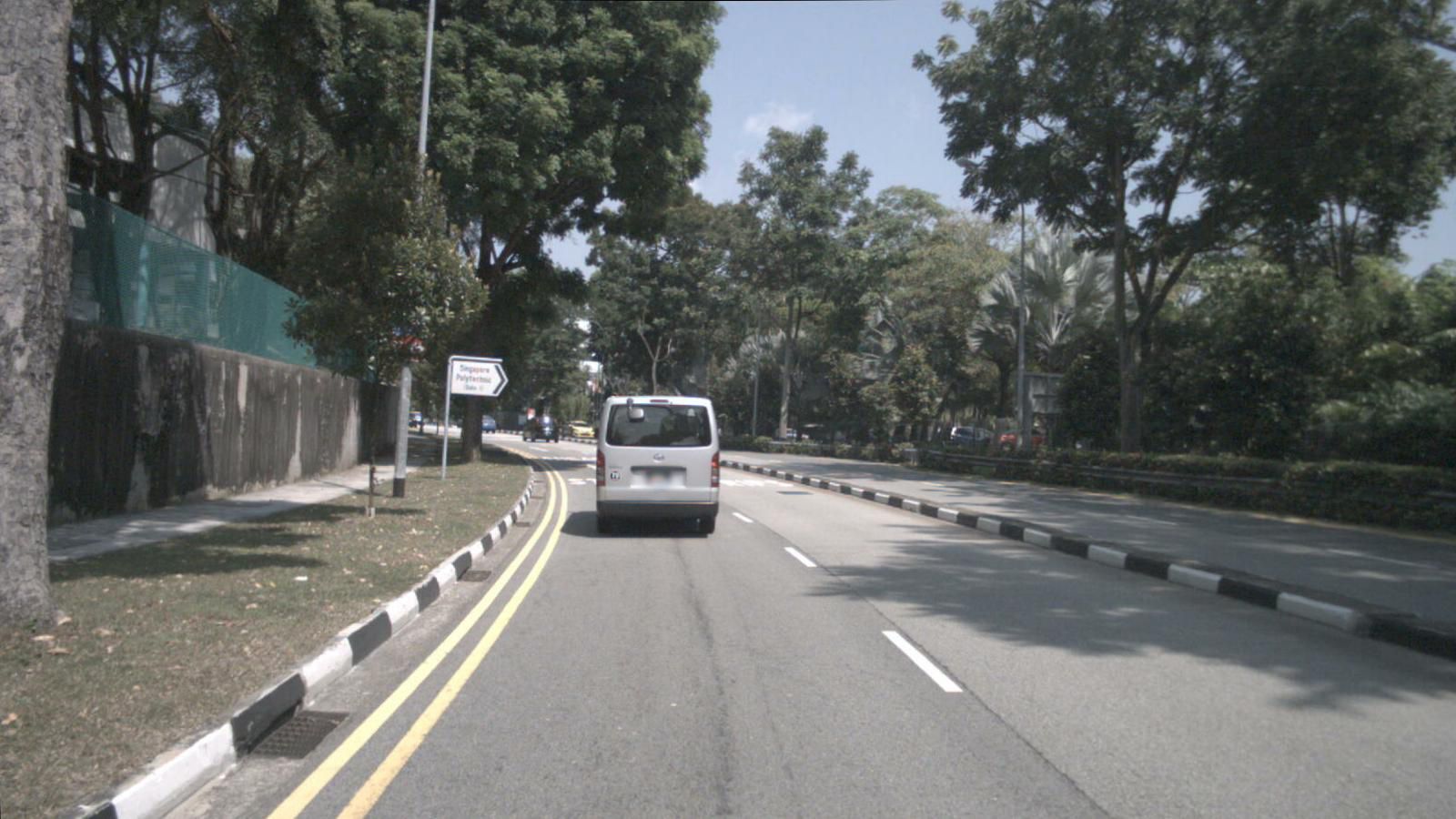
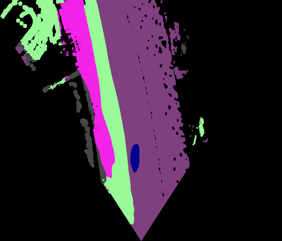
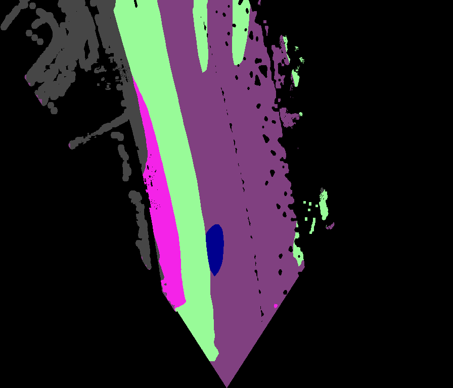
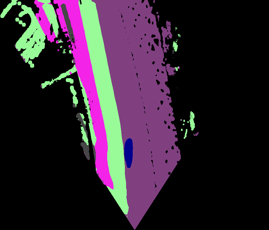
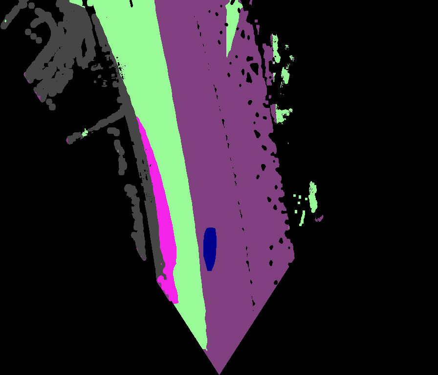
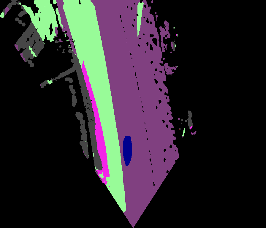
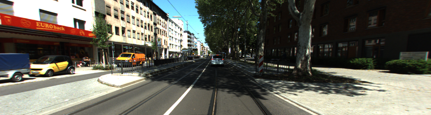
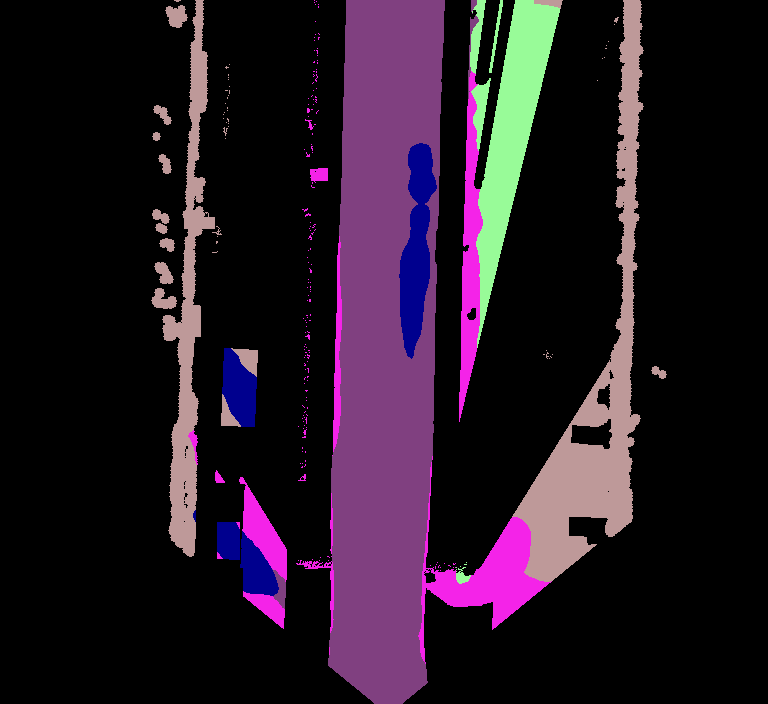
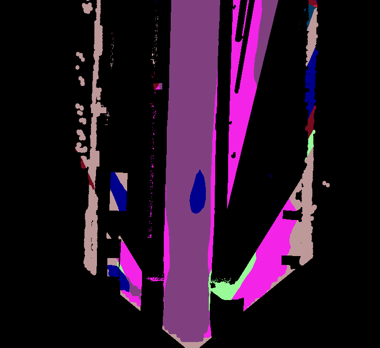
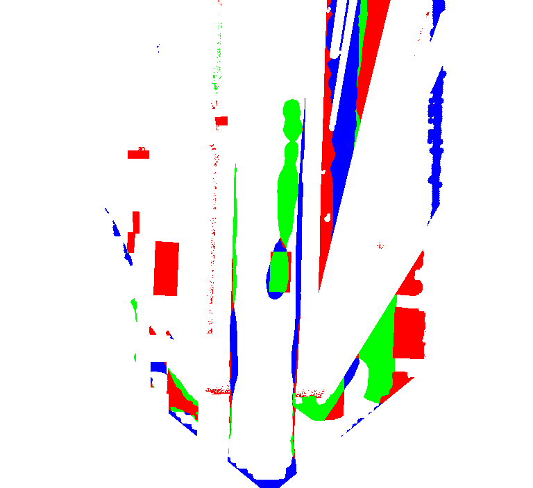
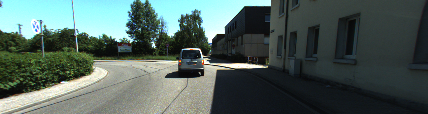
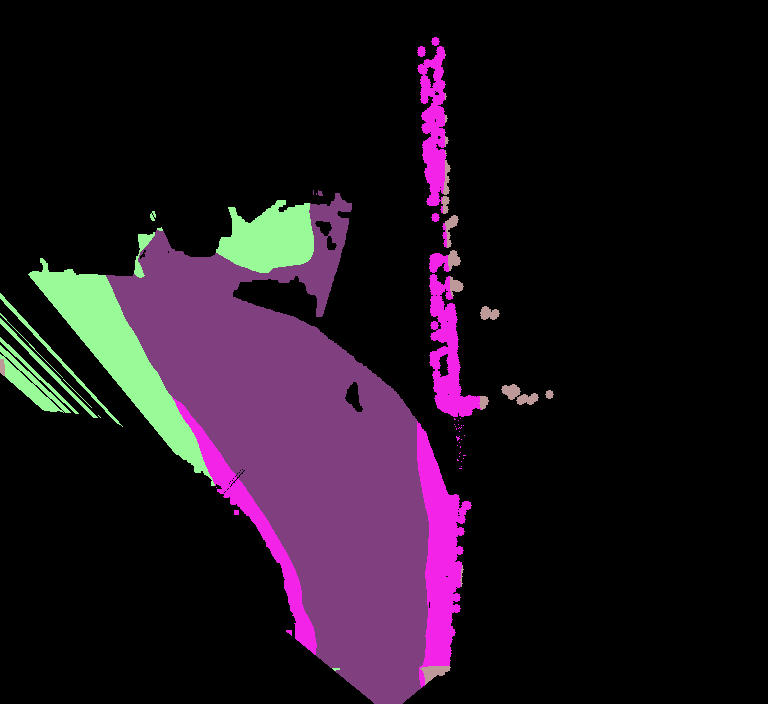
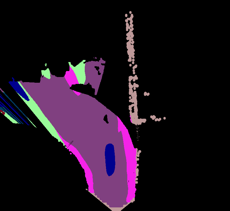
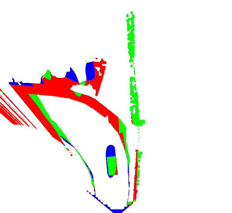
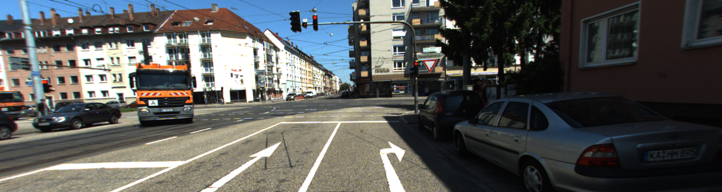
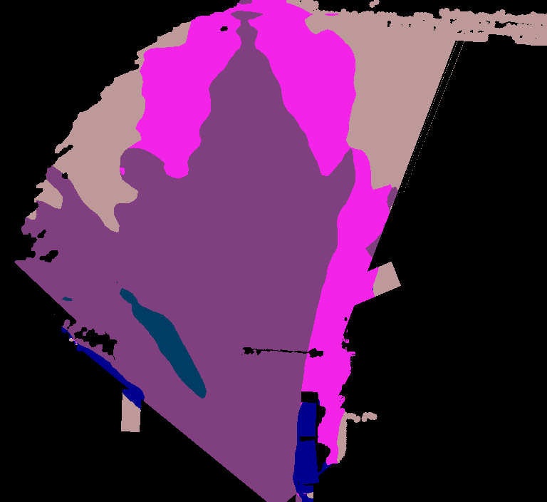
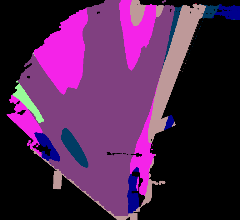
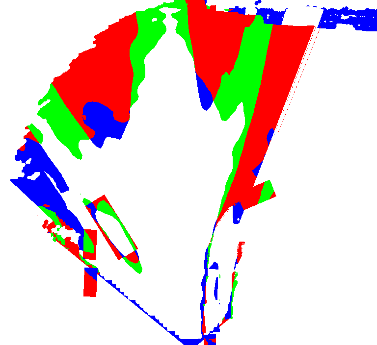
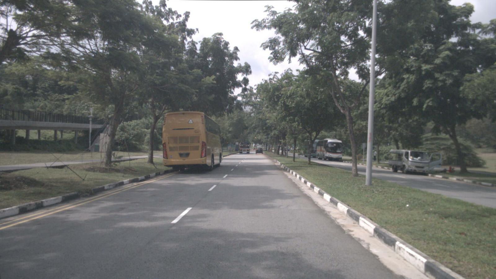
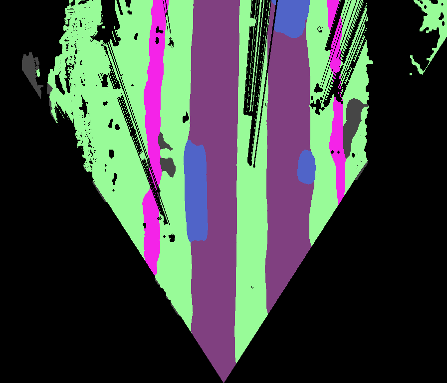
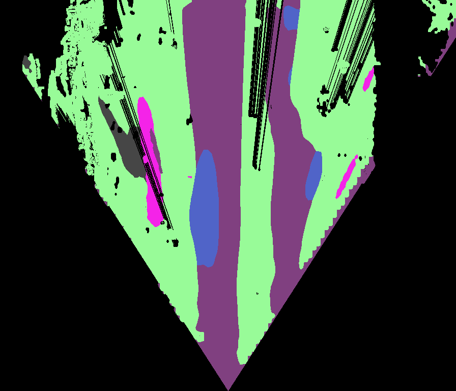
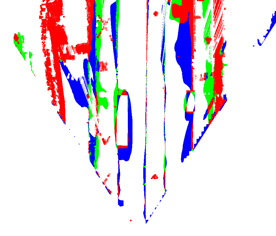
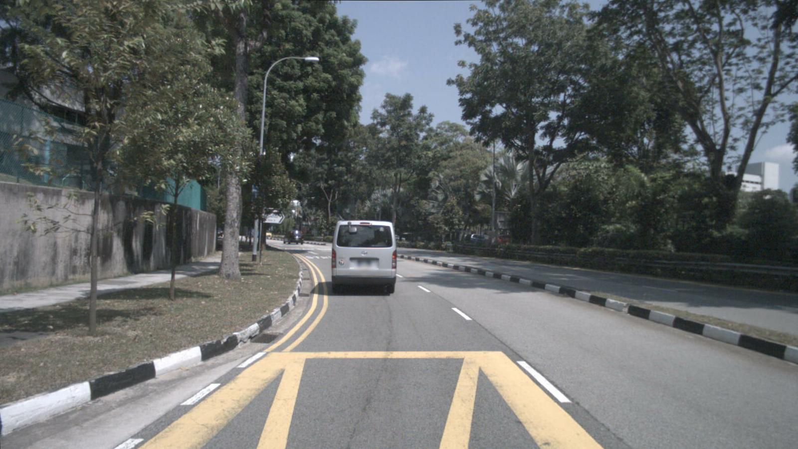
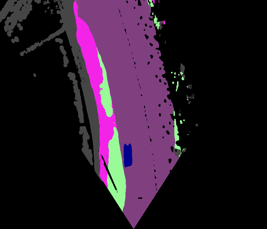
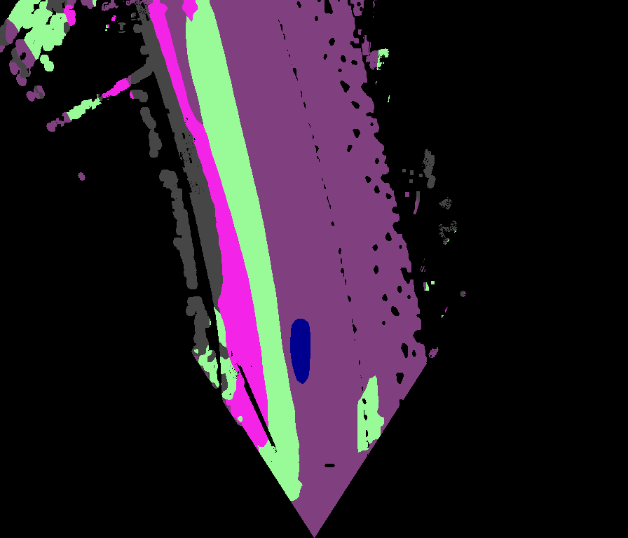
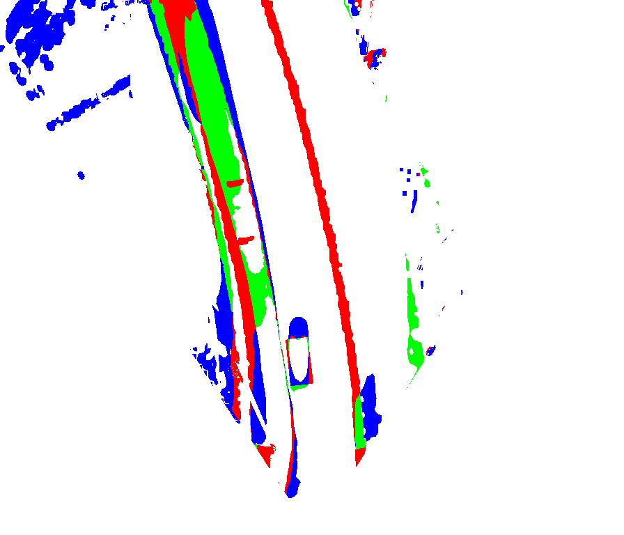
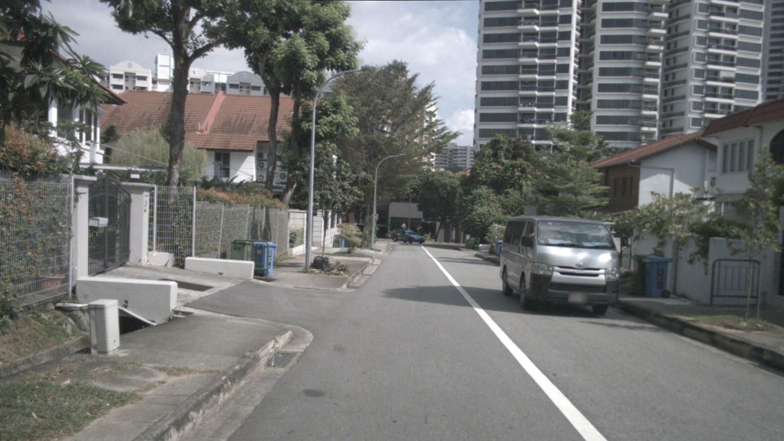
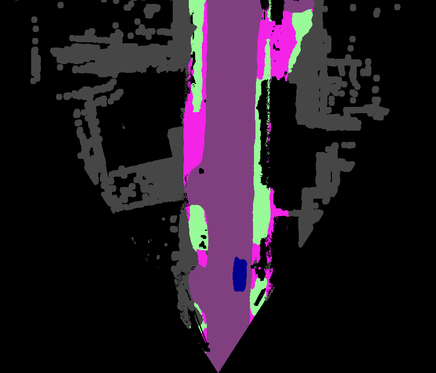
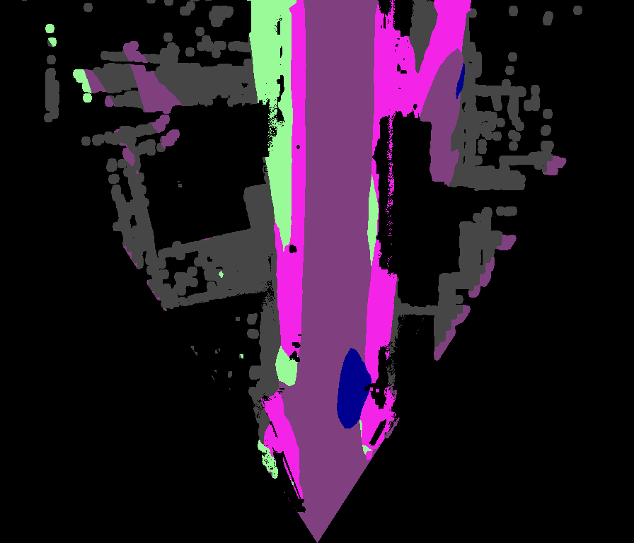
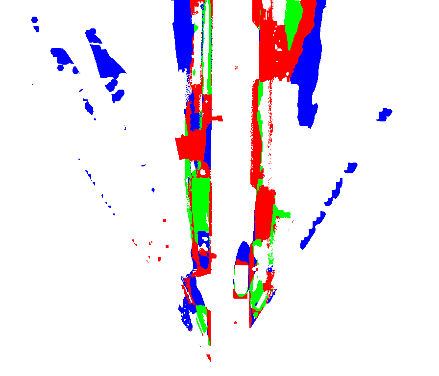
Figure 4 compares frontal inputs, baseline maps, LetsMap predictions, and error/improvement maps. Some examples show better vehicle extents and sensible continuation of terrain or road behind occluders. Other dynamic objects remain stretched radially, especially under the sparse temporal views.
Green marks pixels where LetsMap improves over the comparator, blue where the comparator is better, and red where both are wrong. These selected examples illustrate strengths and failures alongside the complete per-class tables.
4.6 Discussion of Limitations
The implicit geometry assumes a largely static scene, needs diverse camera viewpoints, and depends on photometric consistency. Driving footage violates all three through moving objects, narrow observation baselines, changing illumination, and occlusion. Large ego-motion makes these problems worse.
Explicit dynamic-object handling, more useful camera views, or stereo supervision are suggested remedies. They are not part of the evaluated model, so the paper does not establish robust geometry for arbitrary driving conditions.
5 Conclusion
LetsMap demonstrates that image-based geometric pretraining and temporal reconstruction can reduce the BEV labels needed for competitive semantic maps. Its strongest result is in sparse-label regimes, with a pretrained visual backbone and known camera geometry. Dynamic-scene modeling and the residual gap to stronger fully supervised results remain practical limits.
Supplementary material
The supplementary material examines backbone and patch-size choices, backbone-controlled baselines, an alternative label split, and additional qualitative maps.
S.1 Additional Ablative Experiments
Supplementary ablations test whether the main improvements persist under different model capacities, mask geometry, baseline backbones, and selected labeled subsets.
S.1.1 DINOv2 Backbone Variants
At 1% KITTI-360 labels, DINOv2 ViT-small, base, large, and giant yield 25.55, 28.96, 28.40, and 28.16 mIoU. Base is both smaller and slightly better than the larger variants in this experiment. Limited labels or imperfect transfer of frontal features to BEV are proposed explanations rather than separately verified causes.
| Backbone | vit-s | vit-b | vit-l | vit-g |
|---|---|---|---|---|
| mIoU | 25.55 | 28.96 | 28.40 | 28.16 |
| Patch Size | Road | Side. | Build. | Terr. | Per. | 2-Wh. | Car | Truck | mIoU |
|---|---|---|---|---|---|---|---|---|---|
| 14 | 71.45 | 33.41 | 36.89 | 37.48 | 0.75 | 3.69 | 30.05 | 9.23 | 27.87 |
| 28 | 70.58 | 34.26 | 40.68 | 38.53 | 1.35 | 4.74 | 30.94 | 10.58 | 28.96 |
| 56 | 70.02 | 34.10 | 38.87 | 37.88 | 1.37 | 4.71 | 30.91 | 9.66 | 28.44 |
S.1.2 Masking Patch Size
Mask patches of 14, 28, and 56 pixels produce 27.87, 28.96, and 28.44 mIoU. The 28-pixel setting is selected. Smaller patches may make reconstruction too easy, while larger patches can remove distinguishing object information; the numerical comparison establishes the tested preference, not a universal optimal patch size.
S.1.3 Impact of DINOv2 on Baseline Approaches
Replacing PanopticBEV’s native backbone with DINOv2 produces modest improvements, including 30.42→31.83 mIoU with all BEV labels. The same substitution reduces SkyEye performance, for example 26.94→24.09 at 1% labels and 31.47→27.71 at 5%.
Table S.3 therefore helps separate LetsMap’s architecture and pretraining from simply choosing DINOv2. The comparison still changes the baseline feature interface and uses a frozen replacement backbone; its result concerns these adaptations rather than every possible way to retrain the baselines.
| BEV | Model | FV | PT | Backbone | Road | Side. | Build. | Terr. | Pers. | 2-Wh. | Car | Truck | mIoU |
|---|---|---|---|---|---|---|---|---|---|---|---|---|---|
| 1% | PoBEV | ✗ | - | Native | 60.41 | 20.97 | 24.65 | 23.38 | 0.15 | 0.23 | 21.71 | 1.23 | 19.09 |
| SkyEye | ✓ | ✓ | 69.26 | 33.48 | 32.79 | 39.46 | 0.00 | 0.34 | 32.36 | 7.93 | 26.94 | ||
| PoBEV | ✗ | - | DINOv2 | 62.36 | 21.02 | 27.18 | 24.22 | 0.04 | 0.12 | 17.50 | 0.95 | 19.17 | |
| SkyEye | ✓ | ✓ | 65.13 | 29.56 | 29.02 | 34.22 | 0.78 | 2.87 | 26.04 | 5.12 | 24.09 | ||
| LetsMap | ✗ | ✓ | 70.58 | 34.26 | 40.68 | 38.53 | 1.35 | 4.74 | 30.94 | 10.58 | 28.96 | ||
| 5% | PoBEV | ✗ | - | Native | 64.45 | 27.36 | 30.15 | 31.66 | 0.69 | 0.98 | 29.75 | 6.06 | 23.89 |
| SkyEye | ✓ | ✓ | 72.16 | 37.20 | 34.89 | 42.97 | 4.77 | 9.16 | 40.74 | 9.88 | 31.47 | ||
| PoBEV | ✗ | - | DINOv2 | 67.61 | 30.73 | 30.97 | 32.80 | 0.42 | 0.47 | 25.48 | 5.58 | 24.26 | |
| SkyEye | ✓ | ✓ | 69.84 | 34.19 | 32.80 | 37.13 | 2.54 | 4.74 | 32.49 | 7.93 | 27.71 | ||
| LetsMap | ✗ | ✓ | 73.74 | 39.56 | 42.07 | 41.49 | 2.46 | 6.32 | 34.68 | 14.88 | 31.90 | ||
| 10% | PoBEV | ✗ | - | Native | 66.58 | 30.28 | 31.76 | 34.50 | 1.22 | 3.28 | 33.43 | 7.56 | 26.08 |
| SkyEye | ✓ | ✓ | 73.36 | 38.30 | 37.54 | 44.62 | 4.80 | 9.67 | 42.84 | 10.06 | 32.65 | ||
| PoBEV | ✗ | - | DINOv2 | 68.99 | 33.17 | 35.81 | 34.15 | 0.70 | 1.58 | 29.74 | 10.06 | 26.77 | |
| SkyEye | ✓ | ✓ | 72.19 | 36.18 | 35.26 | 39.84 | 3.78 | 5.61 | 36.95 | 10.44 | 30.03 | ||
| LetsMap | ✗ | ✓ | 74.74 | 39.40 | 43.63 | 43.33 | 2.91 | 6.95 | 37.62 | 18.09 | 33.33 | ||
| 50% | PoBEV | ✗ | - | Native | 69.88 | 33.81 | 33.40 | 40.48 | 2.47 | 4.63 | 38.81 | 9.84 | 29.16 |
| SkyEye | ✓ | ✓ | 73.10 | 39.23 | 38.08 | 45.72 | 4.05 | 10.44 | 44.72 | 12.10 | 33.43 | ||
| PoBEV | ✗ | - | DINOv2 | 73.04 | 37.38 | 37.86 | 41.31 | 1.82 | 3.83 | 37.13 | 14.85 | 30.90 | |
| SkyEye | ✓ | ✓ | 73.66 | 38.85 | 41.49 | 41.73 | 2.90 | 6.99 | 38.43 | 12.42 | 32.06 | ||
| LetsMap | ✗ | ✓ | 74.29 | 38.48 | 43.87 | 42.77 | 2.80 | 5.22 | 37.68 | 15.20 | 32.54 | ||
| 100% | PoBEV | ✗ | - | Native | 70.14 | 35.23 | 34.68 | 40.72 | 2.85 | 5.63 | 39.77 | 14.38 | 30.42 |
| SkyEye | ✓ | ✓ | 73.57 | 39.45 | 38.74 | 46.06 | 3.95 | 9.66 | 45.21 | 10.92 | 33.44 | ||
| PoBEV | ✗ | - | DINOv2 | 73.29 | 37.81 | 40.23 | 42.11 | 1.78 | 3.32 | 38.66 | 17.42 | 31.83 | |
| SkyEye | ✓ | ✓ | 73.51 | 39.13 | 40.04 | 42.08 | 3.17 | 5.90 | 39.29 | 12.72 | 31.98 | ||
| LetsMap | ✗ | ✓ | 74.81 | 38.59 | 42.58 | 43.67 | 3.52 | 6.21 | 38.47 | 15.24 | 32.88 |
S.1.4 BEV Finetuning using SkyEye Split
Using SkyEye’s single predefined labeled subset per budget changes absolute results but retains a low-label benefit. At 1%, LetsMap scores 29.70 versus 27.72 without its pretraining and 28.71 for SkyEye. At 10%, the corresponding values are 35.29, 33.53, and 33.41; Table S.4 also retains the 50% comparison.
| BEV | Model | FV | PT | Epochs | Road | Side. | Build. | Terr. | Pers. | 2-Wh. | Car | Truck | mIoU |
|---|---|---|---|---|---|---|---|---|---|---|---|---|---|
| 1% | PoBEV | ✗ | - | 100 | 61.70 | 17.10 | 27.81 | 26.72 | 0.07 | 0.36 | 21.51 | 0.84 | 19.51 |
| SkyEye | ✓ | ✓ | 72.56 | 34.33 | 36.70 | 41.66 | 0.00 | 0.16 | 33.85 | 10.29 | 28.71 | ||
| LetsMap | ✗ | ✗ | 70.89 | 33.88 | 37.71 | 37.41 | 0.80 | 2.87 | 31.59 | 6.59 | 27.72 | ||
| LetsMap | ✗ | ✓ | 72.94 | 37.79 | 43.70 | 38.29 | 0.87 | 2.57 | 30.62 | 10.86 | 29.70 | ||
| 10% | PoBEV | ✗ | - | 50 | 70.00 | 32.75 | 38.07 | 34.43 | 0.80 | 3.33 | 34.46 | 9.25 | 27.89 |
| SkyEye | ✓ | ✓ | 76.07 | 40.30 | 40.30 | 45.33 | 3.75 | 8.15 | 42.64 | 10.73 | 33.41 | ||
| LetsMap | ✗ | ✗ | 76.69 | 40.41 | 42.55 | 42.17 | 1.33 | 6.57 | 40.46 | 18.06 | 33.53 | ||
| LetsMap | ✗ | ✓ | 74.47 | 41.16 | 46.31 | 43.31 | 5.48 | 8.80 | 41.55 | 21.24 | 35.29 | ||
| 50% | PoBEV | ✗ | - | 30 | 72.09 | 35.64 | 36.64 | 42.41 | 1.61 | 3.92 | 41.41 | 9.77 | 30.44 |
| SkyEye | ✓ | ✓ | 76.43 | 39.89 | 45.22 | 46.64 | 5.10 | 7.93 | 42.43 | 12.30 | 34.49 | ||
| LetsMap | ✗ | ✗ | 75.46 | 39.45 | 42.71 | 39.69 | 3.85 | 5.70 | 41.88 | 17.82 | 33.32 | ||
| LetsMap | ✗ | ✓ | 76.54 | 42.65 | 49.23 | 41.47 | 3.36 | 8.61 | 38.76 | 19.42 | 35.01 |
S.2 Additional Qualitative Results
Figure S.1 shows eight examples across KITTI-360 and nuScenes as supervision increases from 1% to 100%. Predictions often remain similar, while more labels can reduce radial stretching, heading errors, or incorrect use of scene priors. In one example, the sparse-label model mistakes a grass patch for road while better-supervised variants recover it.
These examples show both useful completion of occluded regions and cases where prior knowledge is wrong. They do not establish that all objects are correctly detected or that additional labels are unnecessary.