This controller follows a desired collision-free velocity field while changing its damping near obstacles. It stays compliant in free space, rejects motion toward nearby surfaces, and better resists disturbances in simulation and on a seven-joint Franka arm. The collision theorem has restricted geometry and impact assumptions, and the passivity analysis explicitly allows a bounded nonpassive velocity region. This edition preserves the requested first arXiv version; the publication link points to the later journal article.
I Introduction
A collision-free velocity command does not guarantee that an inertial, compliant robot will follow it after a push. The controller therefore uses both the desired motion and local obstacle geometry to decide which disturbances to resist. Its main tradeoff is compliance away from obstacles versus stronger corrective forces near them.
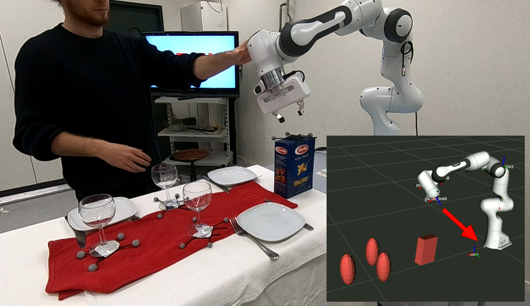
Fig. 1:
The proposed passive obstacle-aware controller lets the robot absorb external disturbances while ensuring collision avoidance.
While tipping over the closed pasta box on this dinner table setup might be acceptable. Yet, the delicate wine glasses demand careful handling to prevent breakage.
I-A Related Work
The background covers interaction-force control and reactive obstacle avoidance.
I-A 1 Force Control
Impedance and damping controllers map motion errors to interaction forces. Variable parameters improve adaptability but need an energy or stability analysis. Previous passive velocity-following designs prioritize the motion direction and can remain too compliant toward an obstacle; energy-tank methods add another way to bound energy but may limit available behavior.
I-A 2 Obstacle Avoidance
Potential fields, navigation functions, geometric motion policies, and velocity modulation provide reactive motion around obstacles. This work assumes an appropriate velocity field is already available and changes the force controller that tracks it. The failure it targets is a disturbance pushing a compliant robot away from that field and into an obstacle.
I-B Contribution
The contributions are an obstacle-sensitive damping matrix, a passivity-region and boundedness analysis, a conditional collision-avoidance argument, a discrete-time parameter analysis, and simulation/hardware comparisons.
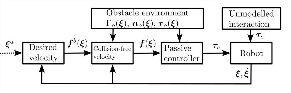
Fig. 2: The desired velocity can result from a learned velocity field or pointing towards a desired attractor . The desired velocity is used to evaluate the obstacle avoidance velocity , fed into the force controller to obtain the control force . In order to achieve collision avoidance, the distance function , the normal direction , and the reference direction are evaluated for each obstacle .
II Preliminaries
The state can represent joint or Cartesian position in at least two dimensions. A continuous vector field supplies desired velocity; the physical system has second-order dynamics.
II-A Obstacle Avoidance
Velocity modulation reduces motion in an obstacle’s reference direction and increases tangential motion. A distance function equals one at the surface and grows outside it. The construction assumes star-shaped obstacles with a suitable internal reference point. This geometric layer supplies the collision-free desired field used by the damping controller.
Equations 1–3
(1)
(2)
(3)
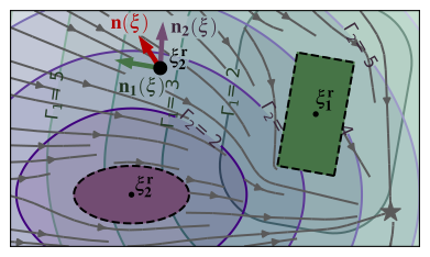
Fig. 3:
The -field is defined individually for each of the obstacles. At each position , we can evaluate the surface normal .
The velocity (gray) avoids collision with the obstacles and converges towards the attractor (star).
II-B Force Control
Rigid-body dynamics and a gravity-compensated damping law connect desired velocity to control force.
II-B 1 Rigid Body Dynamics
The model includes inertia, Coriolis effects, gravity, applied control, and external disturbance force. The energy analysis uses the standard skew-symmetry property of the rigid-body inertia and Coriolis terms.
Equation 4
(4)
II-B 2 Damping Controller
The baseline applies gravity compensation plus D times desired-minus-actual velocity. An orthonormal basis aligns the largest damping direction with the desired motion, while smaller transverse values permit compliance. All damping eigenvalues are positive.
Equations 5–7
(5)
(6)
(7)
II-C Stability Analysis
Passivity compares change in stored energy with supplied input–output power. It is useful for interaction analysis, but a robot accelerating toward a nonzero commanded velocity can inject kinetic energy without an external push. The later result therefore identifies where the passivity inequality holds rather than asserting it at every velocity.
Equation 8
(8)
II-D Problem Statement
The desired velocity must be continuous, bounded, and directed tangentially or outward at obstacle boundaries. These conditions apply to the commanded first-order field. They do not by themselves guarantee that the disturbed second-order robot remains outside an obstacle.
III Obstacle Aware Passivity
The controller blends velocity-following damping with obstacle-oriented damping. A danger weight increases near a surface and depends on the averaged obstacle normal. Positive-definite components and a weight between zero and one keep the blended damping positive definite.
Equations 9–10
(9)
(10)
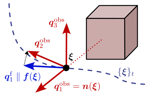
Fig. 4: The damping matrix enforcing desired velocity following has the first basis vector which points along the avoidance velocity . The damping matrix to enforce collision avoidance uses the normal to construct the first direction of the decomposition basis .
III-A Damping for Collision Repulsion
The obstacle component chooses a direction toward nearby surfaces, an orthogonal tracking direction, and corresponding damping strengths.
III-A 1 Normal Direction
Inverse-distance weights combine obstacle normals, emphasizing the closest surfaces. The result approaches the nearest obstacle’s normal at its boundary. Opposing obstacles can cancel the average, so narrow passages require an additional rule.
Equation 11
(11)
III-A 2 Decomposition Matrix
The first basis vector follows the averaged normal; the second follows the component of desired velocity orthogonal to it. Remaining vectors complete an orthonormal basis. Parallel normal/velocity directions permit an arbitrary transverse basis, with equal transverse damping used to avoid dependence on that choice.
Equations 12–13
(12)
(13)
III-A 3 Damping Values
Large normal damping resists motion toward an obstacle, intermediate damping follows the desired velocity, and small remaining values preserve compliance. Interpolating transverse damping as the normal aligns with the velocity helps keep the resulting control force continuous.
Equations 14–15
(14)
(15)
III-A 4 Damping Only Towards Obstacle
Strong normal damping is used when the velocity error requires correction away from the obstacle. Moving away from the surface can remain compliant. Although the selected damping coefficient switches, its multiplying error component is zero at the switch, preserving force continuity in the stated construction.
Equation 16
(16)
III-B Damping for Velocity Preservation
The velocity-following component normally emphasizes the commanded direction. Near opposing surfaces, its eigenvalues are raised so that cancellation of the average normal does not leave a compliant direction toward either obstacle.
Equation 17
(17)
III-C Cluttered Environments
When two nearby surfaces have opposing normals, the obstacle-oriented weight tends to zero while the modified velocity component tends to high isotropic damping. This supplies disturbance resistance in narrow passages without requiring a well-defined averaged normal.
Equations 18–19
(18)
(19)
III-D Damping Parameter Design
The recommended ordering is obstacle damping at least as large as velocity-following damping, both much larger than the positive compliance value. Stronger damping improves rejection but raises forces and can destabilize a sampled implementation if chosen without regard to the update interval.
Equation 20
(20)
III-E Passivity Analysis
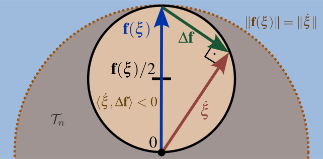
Using kinetic energy as storage, the derivative is external power minus a damping expression involving actual velocity and velocity error. For isotropic damping, the inequality is passive outside a circle in velocity space; a sufficient condition is speed at least as large as the commanded speed. Inside the identified region, the controller may add energy to accelerate toward the command.
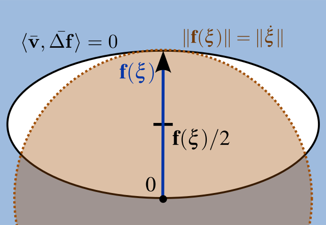
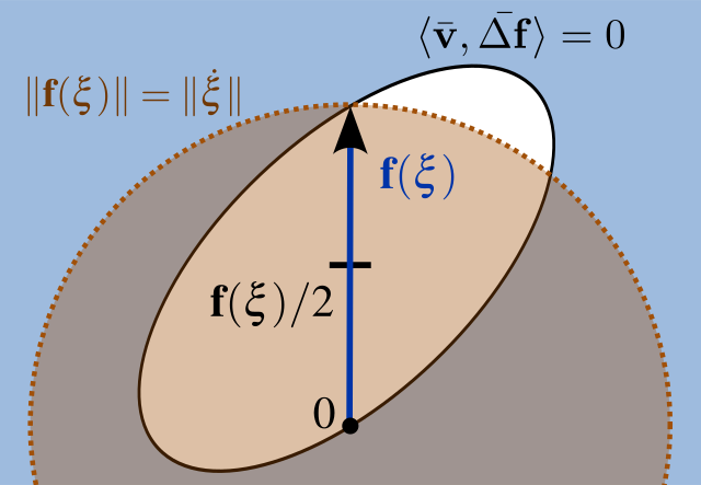
An eigenbasis transformation gives the corresponding elliptical region for anisotropic damping. The paper then states a BIBO-stability result for bounded desired velocity and a continuous finite transformation. This is a velocity-boundedness claim under its model assumptions, not unconditional all-state passivity, target convergence, or collision avoidance. The complete original derivation is retained.
Equations 21–24
(21)
(22)
(23)
(24)
Fig. 5: Analyzing the system in velocity-space yields that the system is passive if it has a velocity larger than the desired velocity , i.e., outside the dashed circle.
However, the system can be non-passive for small velocities when (yellow circle).Equations 25–29
(25)
(26)
(27)
(28)
(29)
((a)),
((b))
Fig. 6:
The stability is ensured even if the controller can temporarily accelerate the system to reach a velocity , which is faster than the desired velocity (white region).
This happens when the eigenvalues of the damping matrix are not uniform (a) or the stretching vectors and are not orthogonal (b).
In both cases, the region of non-passivity is elliptical (black circle).
IV Collision Avoidance
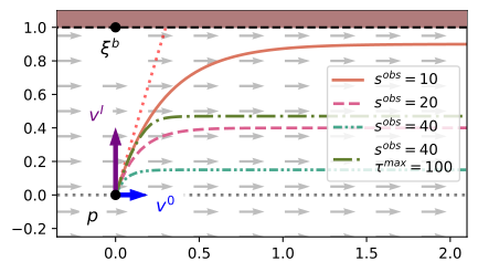
The collision lemma considers a point mass, a flat obstacle, a constant tangential desired velocity, and an impulsive disturbance. The derived displacement bound is proportional to impact speed times mass divided by damping. Sufficient clearance therefore limits the admissible impact magnitude.
Curved surfaces and varying velocity fields fall outside that argument and can still permit drift into obstacles. Force saturation further reduces the impact that can be rejected safely. The paper discusses repulsive-field additions for such cases; it does not establish collision avoidance under arbitrary force, geometry, or actuator limits.
Equations 30–35
(30)
(31)
(32)
(33)
(34)
(35)
Fig. 7: A disturbance occurs of a point-agent at position with velocity after the impact of . A high damping in the direction of the obstacle in the presence of a constant velocity field (gray) ensures collision avoidance. Whereas different damping values and optionally a maximum repulsion force lead to different trajectories.
V Evaluation
The authors’ implementation is compared with a passive velocity-following controller in disturbance simulations and a physical robot experiment.
V-A Qualitative Repulse Rejection
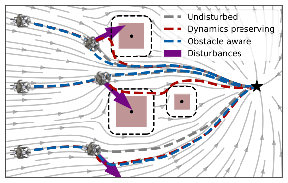
Three simulated scenarios apply pushes toward a single obstacle, between opposing obstacles, and away from a surface. The obstacle-aware controller rejects the first two more strongly, while remaining similarly compliant for the outward push. The baseline collides in the shown inward-disturbance cases.
Fig. 8:
The desired velocity is represented in gray and serves as the input for the force controller. The mobile robot, initially positioned at three different locations, navigates safely towards the attractor (black star) even when confronted with external disturbances (purple arrows) while employing the obstacle-aware controller (blue trajectories). In contrast, the baseline controller (red) results in collisions when disturbances occur close to the robot.
V-B Noise Analysis
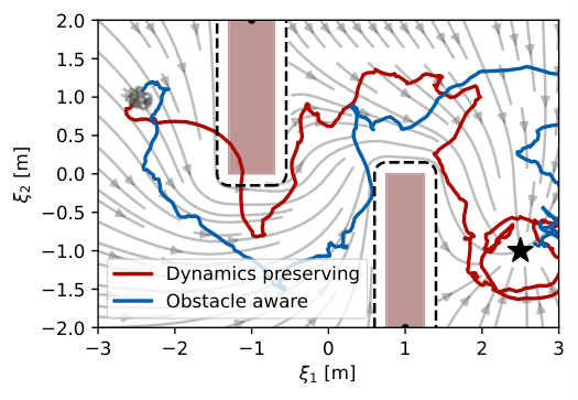
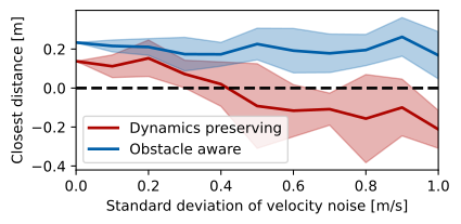
Noise experiments compare the minimum signed surface distance while following a bounded field through two obstacles. Position and velocity corruption test different sources of feedback error; the plots retain the complete tested noise ranges.
((a))Trajectories with a standard deviation of the velocity-noise of 1.0 m/s.
((b))The mean and variance (shaded) of the closest distances over 10 epochs.
Fig. 9: The agent navigates between two elongated obstacles (a) towards the attractor (black star). The agent’s velocity is subjected to white noise, with a mean of zero, and noise variances between and . The robot initiates its trajectory from the starting position , with an initial velocity of zero. It aims to reach the attractor located at .
V-B 1 Velocity Noise Resistance
With zero-mean velocity noise, stronger obstacle-directed damping maintains greater clearance than the baseline. Clearance decreases as noise rises, so the result is improved robustness over the tested range rather than immunity to noise.
V-B 2 Position Noise Resistance
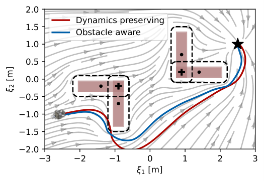
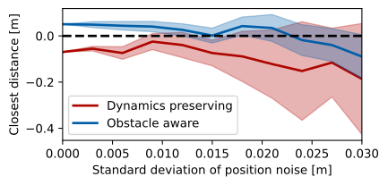
With position noise, the obstacle-aware controller has positive mean minimum clearance for standard deviations below approximately 0.023 m in the reported setup. The baseline’s mean clearance is negative throughout those tests. A positive mean does not imply every trajectory avoids collision.
((a))Trajectories with a standard deviation of the position-noise of 0.0 m.
((b))Closest distances concerning different noise levels over ten epochs.
Fig. 10:
The agent is navigating towards the attractor (black star) between two concave obstacles (a) while being subjected to white noise in its position. The position noise has a mean of zero and various noise variances ranging between and . The robot starts at position , and the attractor is set to .
V-C Obstacle Aware Passivity Using a Robot Arm
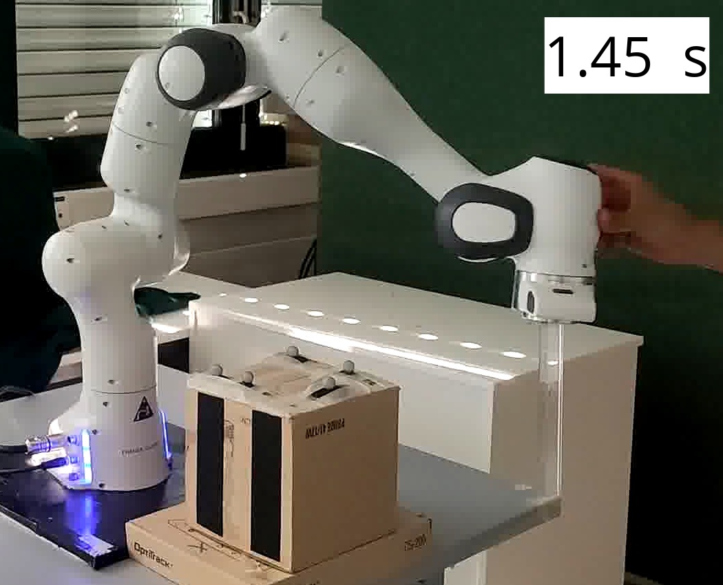
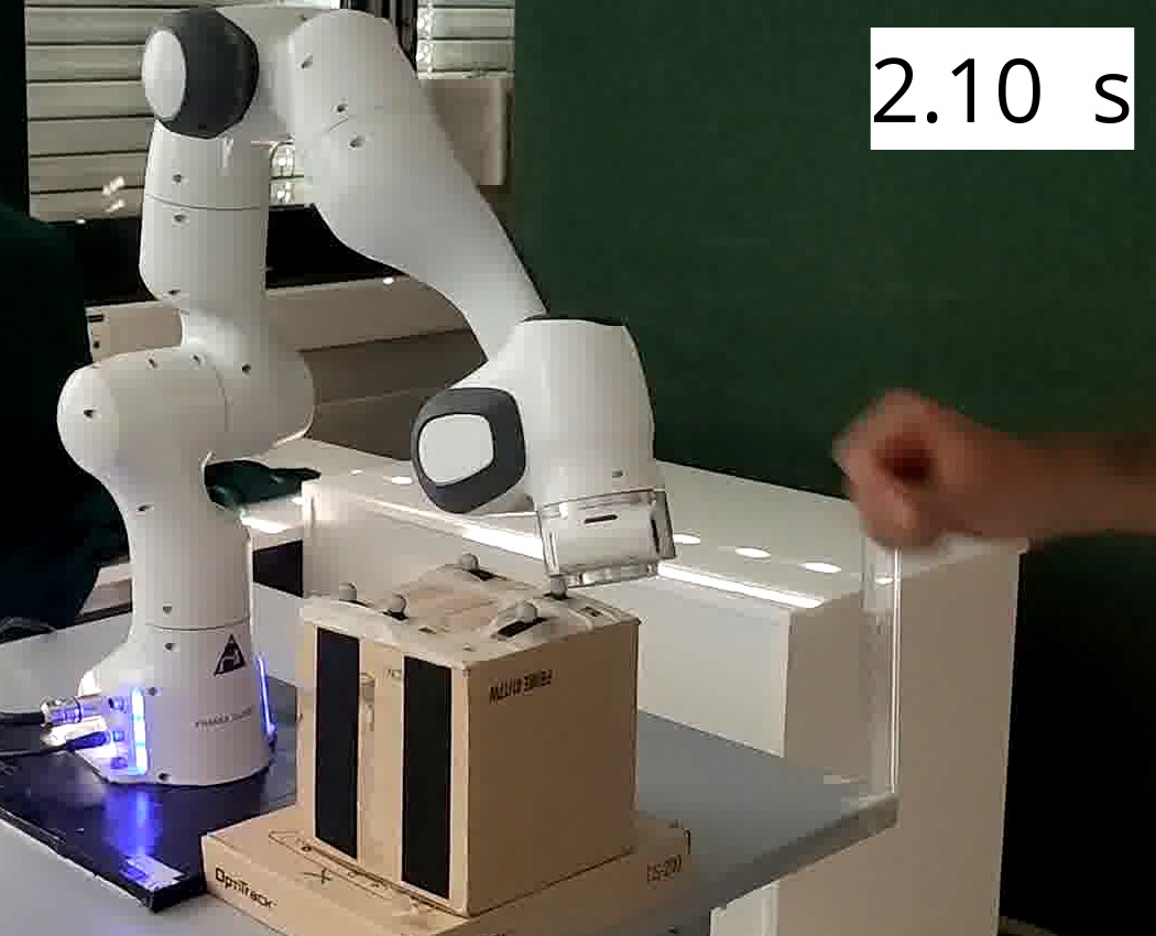
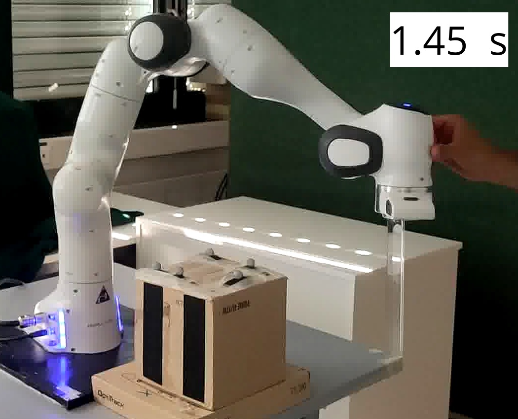
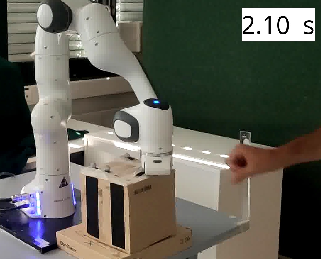
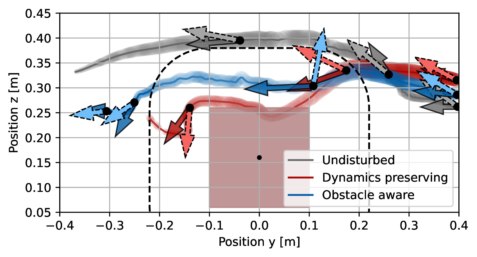
A Franka Panda tracks a desired motion around a 0.16 m box, with a 0.12 m margin and a 500 Hz controller. Optical tracking supplies obstacle position. Ten repeated pushed trials per method compare clearance and peak force with an undisturbed reference.
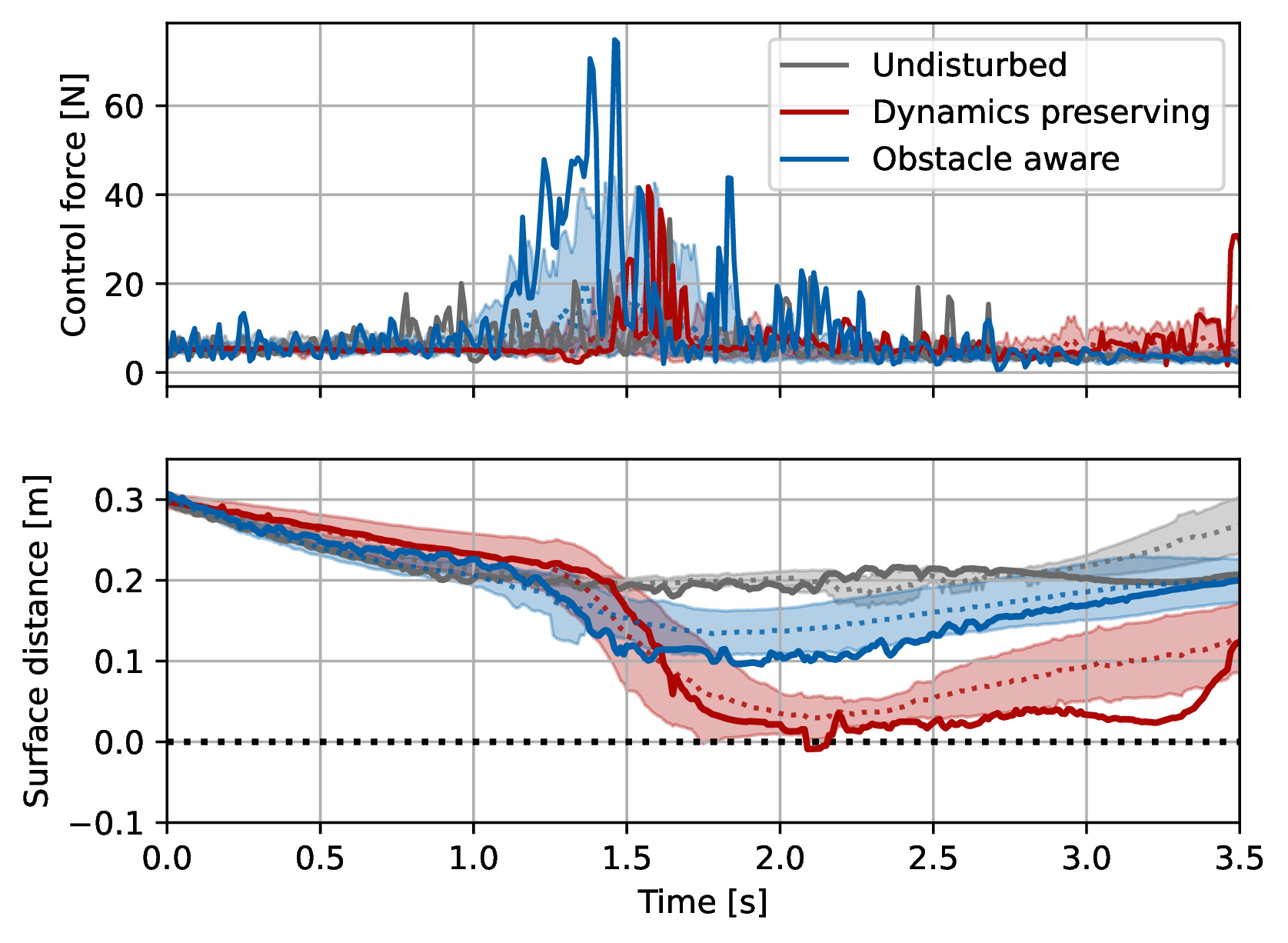
The obstacle-aware trials report about 0.15 m average minimum clearance, compared with below 0.05 m for the velocity-following baseline and several baseline collisions. Improved rejection uses larger momentary forces; Table I preserves their means and standard deviations. Orientation is controlled separately from the translational damping law.
((a))Obstacle-aware controller rejects repulsion and avoids collision
((b))Velocity preserving controller leads to collision with obstacle
((c))The two control methods compared with the undisturbed trajectory. The wider line indicates a higher x-value. The darker arrow is the actual, and the desired velocity is the brighter arrow.
((d))The specific trajectory is represented by a full line, while the average (dashed line) and variance (shaded area) are evaluated over ten epochs. The mean and variance of the control force are evaluated in the logarithmic space.
Fig. 11:
The robot arm, guided by the obstacle-aware passive controller, effectively avoids the disturbance towards the obstacle while maintaining a margin of around the obstacle. The experiment was repeated ten times with a similar disturbance applied to the robot arm in each run.
Equation 36
(36)
Obstacle
Velocity
Undisturbed
Closest Distance [mm]
105 21
18 21
167 9
Maximum Force [N]
4.12 0.25
3.58 0.24
2.86 0.37
TABLE I: The mean and standard deviation of the closest distance and maximum force are evaluated over ten epochs for the proposed obstacle aware controller, and the baseline velocity following controller [10].
The undisturbed trajectory is provided as reference values.
During the experiments, the obstacle-aware damping avoids collision with an increased minimal distance from the obstacle and, hence, a safer trajectory. This is achieved through momentarily higher forces.
VI Discussion
The experiments support selective disturbance rejection near known obstacles. Stability, tracking accuracy, compliance, and collision avoidance are separate properties with different assumptions and tradeoffs.
VI-A Discrete Control Convergence
The controller’s boundedness result does not ensure convergence to a particular position. Adding a proportional term can promote attraction but changes the analyzed system and requires a new stability argument. The desired velocity field is intended to supply convergence behavior in practice.
Equation 37
(37)
VI-B Applicability and Theoretical Analysis
The analysis motivates tank-free damping control with bounded desired velocities, subject to the stated model and matrix assumptions. It does not automatically extend to arbitrary adaptive stiffness or extra feedback terms.
VI-C Point Mass Agents
The analysis treats a point representation of the robot. Evaluating the controller at several points along an arm is suggested for fuller body coverage, but is not a demonstrated whole-body collision guarantee.
VI-D Caution in Obstacle’s Proximity
Obstacle location is assumed known accurately. With uncertain perception, increasing resistance near an estimated surface may conflict with gentle exploration. Combining avoidance with cautious contact is an open direction.
-E Discrete Time Behavior
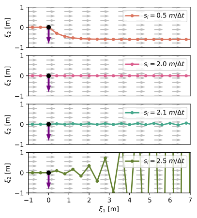
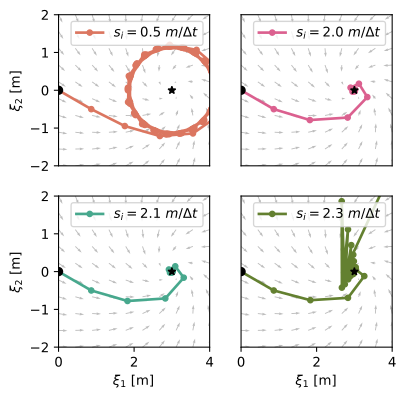
The appendix studies a forward-Euler model. Larger damping improves rapid correction but can create oscillation or divergence when the time step is too large. The paper states the bound sᵢ ≤ 2m/Δt, with m the smallest inertia eigenvalue, and illustrates different choices.
Reading note: in the scalar constant case, the velocity multiplier is 1 − Δt·s/m. At equality it is −1, which is marginal rather than strictly decaying. Strictly inside the bound gives decay for that fixed linear case; the boundary and general state-dependent implementations require care. These sampled-data observations should be kept distinct from the continuous-time analysis.
Fig. 12: An agent has the desired velocity (gray arrow), and a control matrix with damping values equal in all directions and the smallest eigenvalue of the inertia matrix .
The agent is disturbed (purple arrow) position and has a velocity of after the impact.
High damping leads to unstable behavior with increasingly high oscillations. Conversely, the lowest value leads to more deviation from the initial straight line resulting from the higher impedance. The critical value of results in stable behavior with immediate correction to the desired velocity.Equations 38–42
(38)
(39)
(40)
(41)
(42)
Fig. 13: An agent with the desired dynamics of
where is the rotation matrix, and is the mass of the agent. We assume equal damping values .
The controller with a critical stiffness of leads to fast convergence and a stable system. With lower damping (top left), there is a large drift of the system, which converges to a limit cycle.
The high damping of leads to an unstable system.
Interestingly, with damping of in combination with the nonlinear dynamics, we obtain a visibly stable system.
40 references
[1]Lukas Huber, Aude Billard and Jean-Jacques Slotine
“Avoidance of convex and concave obstacles with convergence ensured through contraction”
In IEEE Robotics and Automation Letters4.2IEEE, 2019, pp. 1462–1469
[6]Fares Abu-Dakka and Matteo Saveriano
“Variable impedance control and learning—a review”
In Frontiers in Robotics and AI7Frontiers Media SA, 2020, pp. 590681
[7]Gregory Glosser and Wyatt Newman
“The implementation of a natural admittance controller on an industrial manipulator”
In Proceedings of the 1994 IEEE International Conference on Robotics and Automation, 1994, pp. 1209–1215
IEEE
[8]Perry Li and Roberto Horowitz
“Passive velocity field control of mechanical manipulators”
In IEEE Transactions on robotics and automation15.4IEEE, 1999, pp. 751–763
[9]Elena Gribovskaya, Abderrahmane Kheddar and Aude Billard
“Motion learning and adaptive impedance for robot control during physical interaction with humans”
In 2011 IEEE International Conference on Robotics and Automation, 2011, pp. 4326–4332
IEEE
[10]Klas Kronander and Aude Billard
“Passive interaction control with dynamical systems”
In IEEE Robotics and Automation Letters1.1IEEE, 2015, pp. 106–113
[11]Takuto Fujiki and Kenji Tahara
“Series admittance–impedance controller for more robust and stable extension of force control”
In ROBOMECH Journal9.1Springer, 2022, pp. 23
[12]Yasuo Kishi, Zhi Luo, Fumihiko Asano and Shigeyuki Hosoe
“Passive impedance control with time-varying impedance center”
In Proceedings 2003 IEEE International Symposium on Computational Intelligence in Robotics and Automation. Computational Intelligence in Robotics and Automation for the New Millennium (Cat. No. 03EX694)3, 2003, pp. 1207–1212
IEEE
[13]Alin Albu-Schäffer, Christian Ott and Gerd Hirzinger
“A unified passivity-based control framework for position, torque and impedance control of flexible joint robots”
In The international journal of robotics research26.1Sage Publications Sage CA: Thousand Oaks, CA, 2007, pp. 23–39
[14]Sami Haddadin et al.
“Real-time reactive motion generation based on variable attractor dynamics and shaped velocities”
In 2010 IEEE/RSJ International Conference on Intelligent Robots and Systems, 2010, pp. 3109–3116
IEEE
[15]Stefano Stramigioli, Cristian Secchi, Arjan van Schaft and Cesare Fantuzzi
“Sampled data systems passivity and discrete port-hamiltonian systems”
In IEEE Transactions on Robotics21.4IEEE, 2005, pp. 574–587
[16]Dongjun Lee and Ke Huang
“Passive-set-position-modulation framework for interactive robotic systems”
In IEEE Transactions on Robotics26.2IEEE, 2010, pp. 354–369
[17]Federica Ferraguti, Cristian Secchi and Cesare Fantuzzi
“A tank-based approach to impedance control with variable stiffness”
In 2013 IEEE international conference on robotics and automation, 2013, pp. 4948–4953
IEEE
[18]Klas Kronander and Aude Billard
“Stability considerations for variable impedance control”
In IEEE Transactions on Robotics32.5IEEE, 2016, pp. 1298–1305
[19]Oussama Khatib
“A unified approach for motion and force control of robot manipulators: The operational space formulation”
In IEEE Journal on Robotics and Automation3.1IEEE, 1987, pp. 43–53
[20]Daniel Koditschek and Elon Rimon
“Robot navigation functions on manifolds with boundary”
In Advances in applied mathematics11.4Elsevier, 1990, pp. 412–442
[21]Savvas Loizou and Elon Rimon
“Mobile Robot Navigation Functions Tuned by Sensor Readings in Partially Known Environments”
In IEEE Robotics and Automation LettersIEEE, 2022
[22]Vincent Duindam, Stefano Stramigioli and Jacquelien Scherpen
“Passive compensation of nonlinear robot dynamics”
In IEEE transactions on robotics and automation20.3IEEE, 2004, pp. 480–488
[23]Leena Singh, Harry Stephanou and John Wen
“Real-time robot motion control with circulatory fields”
In Proceedings of IEEE International Conference on Robotics and Automation3, 1996, pp. 2737–2742
IEEE
[24]Sami Haddadin, Rico Belder and Alin Albu-Schäffer
“Dynamic motion planning for robots in partially unknown environments”
In IFAC Proceedings Volumes44.1Elsevier, 2011, pp. 6842–6850
[25]Oliver Brock and Oussama Khatib
“Elastic strips: A framework for motion generation in human environments”
In The International Journal of Robotics Research21.12SAGE Publications Sage UK: London, England, 2002, pp. 1031–1052
[26]Andreea Tulbure and Oussama Khatib
“Closing the loop: Real-time perception and control for robust collision avoidance with occluded obstacles”
In 2020 IEEE/RSJ International Conference on Intelligent Robots and Systems (IROS), 2020, pp. 5700–5707
IEEE
[27]FE Udwadia
“A new perspective on the tracking control of nonlinear structural and mechanical systems”
In Proceedings of the Royal Society of London. Series A: Mathematical, Physical and Engineering Sciences459.2035The Royal Society, 2003, pp. 1783–1800
[29]Ching-An Cheng et al.
“RMP flow: A Computational Graph for Automatic Motion Policy Generation”
In Algorithmic Foundations of Robotics XIII: Proceedings of the 13th Workshop on the Algorithmic Foundations of Robotics 13, 2020, pp. 441–457
Springer
[30]Andrew Bylard, Riccardo Bonalli and Marco Pavone
“Composable geometric motion policies using multi-task pullback bundle dynamical systems”
In 2021 IEEE International Conference on Robotics and Automation (ICRA), 2021, pp. 7464–7470
IEEE
[32]Nathan Ratliff et al.
“Generalized nonlinear and finsler geometry for robotics”
In 2021 IEEE International Conference on Robotics and Automation (ICRA), 2021, pp. 10206–10212
IEEE
[33]Karl Van et al.
“Geometric fabrics: Generalizing classical mechanics to capture the physics of behavior”
In IEEE Robotics and Automation Letters7.2IEEE, 2022, pp. 3202–3209
[34]Christopher Connolly
“Harmonic functions and collision probabilities”
In The International Journal of Robotics Research16.4Sage Publications Sage CA: Thousand Oaks, CA, 1997, pp. 497–507
[35]Lukas Huber, Jean-Jacques Slotine and Aude Billard
“Avoidance of Concave Obstacles through Rotation of Nonlinear Dynamics”
In IEEE Transactions on RoboticsIEEE, 2023
[36]Lukas Huber, Jean-Jacques Slotine and Aude Billard
“Avoiding dense and dynamic obstacles in enclosed spaces: Application to moving in crowds”
In IEEE Transactions on Robotics38.5IEEE, 2022, pp. 3113–3132
[39]Jean-Michel Bony
“Principe du maximum, inégalité de Harnack et unicité du probleme de Cauchy pour les opérateurs elliptiques dégénérés”
In Annales de l’institut Fourier19.1, 1969, pp. 277–304