At a glance
A still image may reveal what an object is, while video reveals how it moves. V-JEPA hides large regions across a video and predicts their learned features from what remains visible. Its target encoder slowly follows the context encoder, and a smaller predictor fills in the missing feature descriptions. No pixel decoder, text labels or pretrained image model supplies pretraining targets. Afterward, supervised task heads can use the frozen encoder for action recognition, motion understanding and image tasks. These results show useful transferable video features; the masked task is not restricted to predicting the future, and this paper does not train an action-conditioned robot planner.
1 Introduction
The study revisits feature prediction with modern video transformers, larger datasets and masked modeling. Pretraining uses about two million public videos. The resulting features work particularly well when a task requires temporal distinctions, and adapt with fewer labels than the compared pixel-prediction methods. Frozen evaluation still trains a task-specific head; keeping the encoder fixed is different from having no downstream supervision.
2 Related Works
Slow Features.
Slow-feature methods make nearby frames have similar representations. V-JEPA instead learns a predictor between masked and target regions, allowing related representations to differ in ways explained by position and context.
Predictive Features.
Earlier feature predictors often froze a pretrained encoder or added supervised or contrastive objectives. V-JEPA jointly learns its encoder and predictor through masked-feature regression, with asymmetric updates to address collapse.
Advances in Self-Supervised Learning.
Vision transformers make it practical to omit masked tokens and process the remainder. Prior image methods supply the momentum-target design, while attentive pooling improves how frozen features are evaluated. The recipe combines these advances rather than claiming every component is new.
Feature Prediction versus Pixel Reconstruction.
Feature targets can ignore some unpredictable pixel detail, letting capacity support transferable visual structure. The experiments test this benefit in video. Which details are ignored is learned and influenced by masking and data; the objective alone does not identify all task-relevant factors.
3 Methodology: Video-JEPA
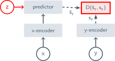
A video encoder represents visible context, and a predictor estimates the features of hidden regions using their positions. The target branch processes the complete clip to supply contextualized targets. This extends image JEPA to spatiotemporal patches.
3.1 Training Objective
The loss averages absolute differences between predicted features and target features. Only the context encoder and predictor receive gradients. The target encoder instead follows an exponential moving average, and its outputs are treated as fixed targets within each optimization step. These asymmetries make the tested training recipe work.
Equations 1
| (1) |
Theoretical motivation.
The motivation analyzes scalar features with an ideal optimal predictor: absolute-error prediction selects a conditional median. Reducing uncertainty in target features motivates informative context representations. The argument neglects several practical dynamics and supplies intuition for the momentum-target design, rather than a general proof that arbitrary JEPA training avoids collapse.
Equations
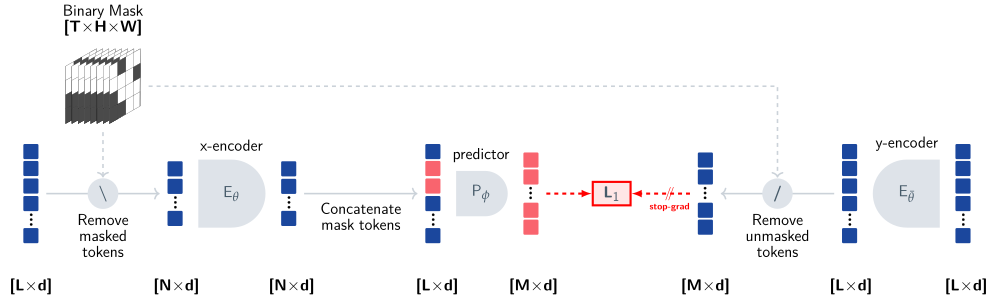
3.2 Prediction Task: Predicting y from x
Masks hide continuous spatial blocks throughout the clip’s temporal extent, reducing easy copying between nearby frames. Short-range and long-range block patterns create complementary tasks; their union masks about 90% of tokens on average. Visible context can occur throughout the video, so this is generally noncausal masked prediction.
3.3 Network Parameterization
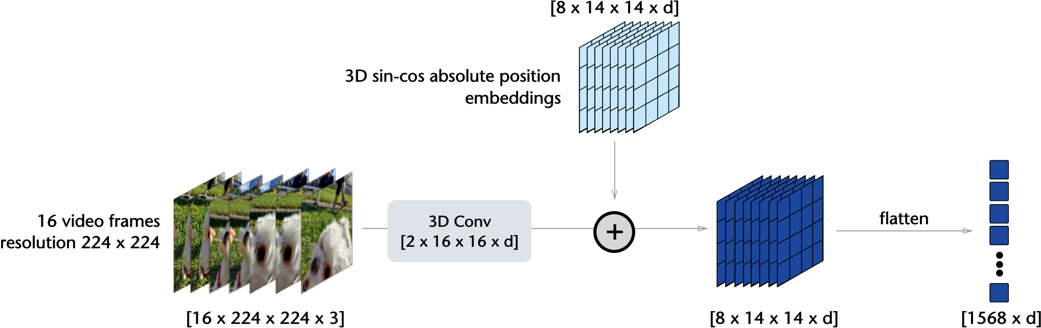
The encoder divides each clip into tokens covering two frames and 16-by-16 pixels. Only visible tokens enter the context encoder. A narrower transformer combines those features with position-marked mask tokens to predict missing features; full-clip target encoding happens before target masking.
3.4 Pretraining Data and Evaluation Setup
Pretraining.
VideoMix 2M combines HowTo 100M, Kinetics and Something-Something-v 2 videos, removing stated overlaps with downstream validation sets. Three encoder configurations vary model size and spatial resolution. All are trained from video without an image-pretraining stage.
Evaluations.
Kinetics emphasizes action recognition, Something-Something-v 2 requires finer motion distinctions, and AVA tests action localization. Static-image benchmarks test transferred object, scene and fine-grained recognition. Evaluations distinguish frozen encoders from end-to-end fine-tuning.
4 What Matters for Learning Representations from Video?
The controlled studies vary prediction targets, pretraining data, pooling and masking. These factors affect different parts of the pipeline and help explain why a headline benchmark gain cannot be attributed to the loss alone.
4.1 Predicting Representations versus Pixels
Matched encoder configurations trained for the same iteration count favor feature prediction over pixel prediction in the reported frozen and fine-tuned tests. Learning-rate and weight-decay sweeps are performed for both objectives.
4.2 Pretraining Data Distribution
Combining datasets improves average performance across tasks under the fixed training budget. A dataset mixture that is best on average is not necessarily best for each benchmark: target-task similarity and visual diversity both matter.
| Frozen Evaluation | |||||
|---|---|---|---|---|---|
| K400 | SSv2 | ||||
| (1611) | (1611) | ||||
| Method | Arch. | Avg. | Att. | Avg. | Att. |
| V-JEPA | ViT-L/16 | 56.7 | 73.7 | 50.1 | 66.2 |
4.3 Evaluation: Attentive Probing
An attentive probe learns how to combine frozen token features instead of simply averaging them. Cross-attention and a small neural head substantially improve measured performance for V-JEPA and several baselines. These scores measure features plus the specified supervised probe, not linear separability alone.
4.4 Prediction Task: Predicting y from x
Continuous multi-block masks outperform the tested random-tube and causal masks. Easy spatial or temporal leakage weakens the learning task. Restricting context to early frames also reduces these downstream scores, so successful representation learning here should not be equated with a strictly causal forecasting objective.
| Frozen Evaluation | |||
| K400 | SSv2 | IN1K | |
| Masking | (1611) | (1611) | |
| random-tube[0.9] | 51.5 | 46.4 | 55.6 |
| causal multi-block[6] | 61.3 | 49.8 | 66.9 |
| causal multi-block[12] | 71.9 | 63.6 | 72.2 |
| multi-block | 72.9 | 67.4 | 72.8 |
| Frozen Evaluation w/ Att. Pooling | Fine-Tuning | ||||||||||
| #Samples | K400 | SSv2 | AVA | IN1K | Places205 | iNat21 | K400-ft | SSv2-ft | |||
| Method | Arch. | Seen | Iter. | (1683) | (1623) | (1653) | (1623) | ||||
| Methods pretrained using pixel prediction | |||||||||||
| OmniMAE | ViT-L/16 | 2400M | 1170K | 65.6 | 60.6 | 14.4 | 75.1 | 59.8 | 66.1 | 84.0 | 74.2 |
| VideoMAE | ViT-L/16 | 410M | 400K | 77.8 | 65.5 | 21.6 | 71.1 | 59.3 | 64.6 | 85.4 | 74.3 |
| Hiera | Hiera-L | 770M | 1500K | 75.5 | 64.2 | 15.8 | 68.9 | 58.5 | 56.9 | 87.3 | 75.1 |
| V-JEPA | ViT-L/16 | 270M | 90K | 80.8 | 69.5 | 25.6 | 74.8 | 60.3 | 67.8 | 85.6 | 75.1 |
| Video Tasks | Image Tasks | ||||||||
| K400 | SSv2 | AVA | IN1K | Places205 | iNat21 | ||||
| Method | Arch. | Params. | Data | (1683) | (1623) | ||||
| Methods pretrained on Images | |||||||||
| I-JEPA | ViT-H/16512 | 630M | IN22K | 79.7 | 50.0 | 19.8 | 84.4 | 66.5 | 85.7 |
| OpenCLIP | ViT-G/14 | 1800M | LAION | 81.8 | 34.8 | 23.2 | 85.3 | 70.2 | 83.6 |
| DINOv2 | ViT-g/14 | 1100M | LVD-142M | 83.4 | 50.6 | 24.3 | 86.2 | 68.4 | 88.8 |
| Methods pretrained on Videos | |||||||||
| MVD | ViT-L/16 | 200M | IN1K+K400 | 79.4 | 66.5 | 19.7 | 73.3 | 59.4 | 65.7 |
| OmniMAE | ViT-H/16 | 630M | IN1K+SSv2 | 71.4 | 65.4 | 16.0 | 76.3 | 60.6 | 72.4 |
| VideoMAE | ViT-H/16 | 630M | K400 | 79.8 | 66.2 | 20.7 | 72.3 | 59.1 | 65.5 |
| VideoMAEv2 | ViT-g/14 | 1100M | Un.Hybrid | 71.2 | 61.2 | 12.9 | 71.4 | 60.6 | 68.3 |
| Hiera | Hiera-H | 670M | K400 | 77.0 | 64.7 | 17.5 | 71.4 | 59.5 | 61.7 |
| V-JEPA | ViT-L/16 | 200M | VideoMix2M | 80.8 | 69.5 | 25.6 | 74.8 | 60.3 | 67.8 |
| ViT-H/16 | 630M | 82.0 | 71.4 | 25.8 | 75.9 | 61.7 | 67.9 | ||
| ViT-H/16384 | 630M | 81.9 | 72.2 | 25.0 | 77.4 | 62.8 | 72.6 | ||
5 Comparison with Prior Work
Comparisons first control encoder size, then compare larger published configurations, and finally reduce the amount of downstream labeled data. Each protocol answers a different question about the features.
5.1 Comparison with Pixel Prediction
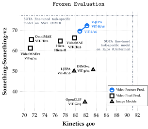
Against similarly sized pixel-prediction systems, V-JEPA improves most frozen video and image evaluations and remains competitive after full fine-tuning. The ImageNet comparison has a small exception: an image-and-video-trained OmniMAE model scores slightly higher than video-only V-JEPA. Pretraining exposure differs across released baselines.
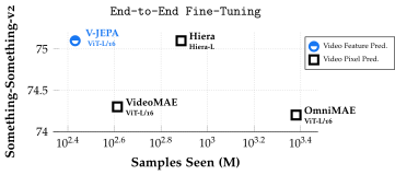
5.2 Comparison with State-of-the-Art
The broader comparison includes much larger image and video models with differing data and supervision. It establishes a useful empirical reference, not an isolated test of one architectural choice.
| Frozen Evaluation | |||||||
| K400 | SSv2 | ||||||
| (1683) | (1623) | ||||||
| 5% | 10% | 50% | 5% | 10% | 50% | ||
| Method | Arch. | (29 samples per class) | (58 samples per class) | (287 samples per class) | (48 samples per class) | (96 samples per class) | (440 samples per class) |
| MVD | ViT-L/16 | 62.6 0.2 | 68.3 0.2 | 77.2 0.3 | 42.9 0.8 | 49.5 0.6 | 61.0 0.2 |
| VideoMAE | ViT-H/16 | 62.3 0.3 | 68.5 0.2 | 78.2 0.1 | 41.4 0.8 | 48.1 0.2 | 60.5 0.4 |
| VideoMAEv2 | ViT-g/14 | 37.0 0.3 | 48.8 0.4 | 67.8 0.1 | 28.0 1.0 | 37.3 0.3 | 54.0 0.3 |
| V-JEPA | ViT-H/16 | 67.0 0.2 | 72.1 0.1 | 80.2 0.2 | 51.9 0.3 | 57.5 0.4 | 67.3 0.2 |
| ViT-H/16384 | 68.2 0.2 | 72.8 0.2 | 80.6 0.2 | 54.0 0.2 | 59.3 0.5 | 67.9 0.2 | |
Comparison with video models.
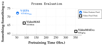
V-JEPA improves the reported frozen-task results over the selected video baselines, especially on motion-sensitive recognition. Reported wall-clock advantages depend on the actual schedules and implementations, including any teacher-pretraining stages.
Comparison with image models.
Video pretraining helps on motion distinctions that static-image encoders struggle with. Image models can remain stronger on appearance-heavy Kinetics classification or image recognition. Attentive probing also improves their scores; no single task provides a universal ordering of encoders.
5.3 Label-efficiency
Frozen heads are trained with 5%,10% and 50% of downstream labels, using three random splits. V-JEPA’s relative advantage grows as labels become scarce. Pretraining remains self-supervised, but every low-shot score still depends on the available task labels.
6 Evaluating the Predictor
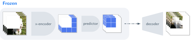
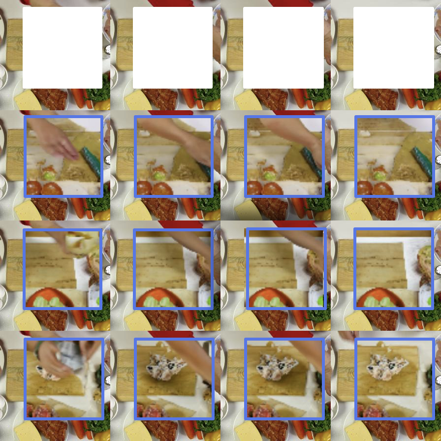
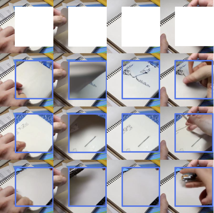
A separately trained diffusion decoder translates frozen feature predictions into illustrative videos. Consistent object layout and movement across sampled decodes suggest grounded predictive features. The visualizer is added after V-JEPA training, and its examples are qualitative evidence rather than a general proof of physical understanding.
7 Conclusion
Masked-feature prediction produces transferable video representations, with particularly strong tested motion and low-label performance. The demonstrated outcome is a reusable perceptual encoder. Action conditioning, closed-loop control and unrestricted long-horizon forecasting lie beyond this paper’s experiments.
Appendix A Extended Related Works
The extended review locates V-JEPA among image and video approaches with different supervision and prediction targets.
Weakly-Supervised Learning from Static Images
Image–text methods use naturally paired captions as weak supervision. Their strong frozen features are relevant baselines, but their data and training signals differ from video-only self-supervision.
Self-Supervised Learning from Static Images
Image self-supervision includes transformation invariance, denoising and learned feature prediction. Some strong systems combine these objectives and use much larger curated image collections.
Weakly-Supervised Learning from Videos
Video–language systems can exploit audio transcripts or accompanying captions. V-JEPA’s pretraining excludes that text supervision, which matters when comparing data efficiency or task coverage.
Self-Supervised Learning from Videos
Temporal ordering, optical flow and interpolation supply alternative video learning signals. Masked latent prediction is one choice among these, not the only way to extract supervision from time.
Appendix B Extended Description of V-JEPA
The extended method specifies how clips become tokens, how masks split context and targets, and which networks receive updates.
Input.
A default clip samples 16 frames with temporal stride 4, spanning roughly two seconds. A three-dimensional convolution converts it into 1568 spatiotemporal tokens at 224-pixel resolution, and positional embeddings retain their locations.
V-JEPA .
The context branch sees unmasked tokens; learned mask tokens request target locations from the predictor. The momentum target branch processes the full clip once. Absolute feature error trains the context encoder and predictor before the target weights are averaged toward them.
Equation 2
| (2) |
Multi-Mask Prediction.
Two masks share one full-clip target computation. Context encoding and prediction are repeated for each mask, amortizing part of the training cost.
Appendix C Pretraining details
The retained table records the complete pretraining configurations, including schedules, resolution and model size.
| Hyper-parameter | ViT-L/16224 | ViT-H/16224 | ViT-H/16384 |
|---|---|---|---|
| data | |||
| datasets | VideoMix2M | VideoMix2M | VideoMix2M |
| resolution | 224 | 224 | 384 |
| num_frames | 16 | 16 | 16 |
| temporal_stride | 4 | 4 | 4 |
| horizontal_flip | true | true | true |
| random_resize_scale | (0.3, 1.0) | (0.3, 1.0) | (0.3, 1.0) |
| random_resize_aspect_ratio | (0.75, 1.35) | (0.75, 1.35) | (0.75, 1.35) |
| masking | |||
| block_aspect_ratio | (0.75, 1.5) | (0.75, 1.5) | (0.75, 1.5) |
| shortrange_mask_num_blocks | 8 | 8 | 8 |
| shortrange_mask_spatial_scale | 0.15 | 0.15 | 0.15 |
| longrange_mask_num_blocks | 2 | 2 | 2 |
| longrange_mask_spatial_scale | 0.7 | 0.7 | 0.7 |
| optimization | |||
| batch_size | 3072 | 3072 | 2400 |
| total_number_of_iterations | 90000 | 90000 | 90000 |
| warmup_iterations | 12000 | 12000 | 12000 |
| lr | 6.25e-4 | 6.25 | 6.25 |
| start_lr | 2 | 2 | 2 |
| final_lr | 1 | 1 | 1 |
| start_momentum | 0.998 | 0.998 | 0.998 |
| final_momentum | 1.0 | 1.0 | 1.0 |
| start_weight_decay | 0.04 | 0.04 | 0.04 |
| final_weight_decay | 0.4 | 0.4 | 0.4 |
| scheduler_scale_factor | 1.25 | 1.25 | 1.25 |
| architecture | |||
| patch_size | 16 | 16 | 16 |
| tubelet_size | 2 | 2 | 2 |
| pred_depth | 12 | 12 | 12 |
| pred_embed_dim | 384 | 384 | 384 |
| hardware | |||
| dtype | bfloat16 | bfloat16 | bfloat16 |
| accelerator | A100 80G | A100 80G | A100 80G |
Architectures.
All models use 16-frame clips and a 12-block,384-wide predictor. Encoders vary in size and spatial resolution. Pretraining does not use a classification token.
Optimization.
AdamW trains for 90,000 iterations. Learning rate, weight decay and momentum schedules are computed for a longer hypothetical run, then truncated. This schedule modification is an explicit part of the successful recipe.
Masking.
The two mask families use several smaller blocks or fewer larger blocks, extending through time. They share a high effective masking ratio but vary the spatial prediction problem.
Appendix D Evaluation details
D.1 Frozen classification
| Hyper-parameter | K400 | SSv2 | IN1K | Place205 | iNat21 |
|---|---|---|---|---|---|
| data | |||||
| num_clips | 8 | 1 | N.A. | N.A. | N.A. |
| num_frames | 16 | 16 | N.A. | N.A. | N.A. |
| temporal_stride | 4 | 4 | N.A. | N.A. | N.A. |
| horizontal_flip | true | true | true | true | true |
| random_resize_scale | (0.08, 1.0) | (0.08, 1.0) | (0.08, 1.0) | (0.08, 1.0) | (0.08, 1.0) |
| random_resize_aspect_ratio | (0.75, 1.33) | (0.75, 1.33) | (0.75, 1.33) | (0.75, 1.33) | (0.75, 1.33) |
| auto_augment | false | false | true | true | true |
| optimization | |||||
| batch_size | 256 | 256 | 1024 | 1024 | 1024 |
| epochs | 20 | 20 | 20 | 20 | 20 |
| lr | 1e-3 | 1e-3 | 1e-3 | 1e-3 | 1e-3 |
| final_lr | 0 | 0 | 0 | 0 | 0 |
| weight_decay | 0.01 | 0.01 | 0.01 | 0.01 | 0.01 |
Attentive Probing.
A learned query attends to frozen encoder tokens, followed by a small nonlinear network and classifier. Only this probe is trained for the downstream classification task. Its capacity matters when interpreting a frozen-backbone score.
Equation
Optimization.
Probe training uses AdamW, a cosine schedule and task-specific augmentation. The appendix table supplies the settings rather than treating the probe as a parameter-free readout.
Extension to multiple clips.
Several clips sampled across a video are encoded separately, then their features are combined by the probe. Test-time spatial views are averaged. This increases temporal coverage and evaluation work.
Application of video models to images.
A static image is duplicated across frames to fit the video tokenizer. This is an evaluation interface choice, not additional temporal information.
Application of image models to videos.
Image encoders process frames independently; their token features are then combined by the same kind of attentive probe. Any temporal integration in this baseline occurs in the task head.
D.2 Frozen detection
AVA evaluation uses externally pretrained region proposals and a supervised classifier above frozen features. The mAP score therefore reflects the complete stated detection pipeline, not an unsupervised object detector learned by V-JEPA alone.
| Hyper-parameter | ViT-L/16 | ViT-H/16 |
|---|---|---|
| out_layers | [18, 20, 22, 24] | [26, 28, 30, 32] |
| batch_size | 64 | 64 |
| epochs | 30 | 30 |
| opt | AdamW | AdamW |
| opt_eps | 0.00000001 | 0.00000001 |
| momentum | 0.9 | 0.9 |
| weight_decay | 0.05 | 0.05 |
| lr | 0.0001 | 0.0001 |
| warmup_lr | 0.000001 | 0.000001 |
| min_lr | 0.000001 | 0.000001 |
| warmup_epochs | 2 | 2 |
| warmup_steps | 1 | 1 |
D.3 Finetuning
End-to-end fine-tuning updates the encoder and classifier with task labels. Its layer-wise learning-rate decay and augmentation recipe are separate from frozen evaluation.
| Hyper-parameter | K400 | SSv2 | ||
|---|---|---|---|---|
| data | ||||
| num_segments | 1 | |||
| num_frames | 16 | |||
| sampling_rate | 4 | |||
| resolution | 224 | |||
| model | ||||
| model_name | ViT-L/16 | ViT-H/16 | ViT-L/16 | ViT-H/16 |
| drop_path | 0.1 | 0.2 | 0.2 | 0.2 |
| head_drop_rate | 0. | 0. | 0.5 | 0.5 |
| optimization | ||||
| batch_size | 256 | 1024 | 256 | 256 |
| epochs | 35 | 25 | 15 | 15 |
| opt | adamw | |||
| opt_eps | 0.00000001 | |||
| momentum | 0.9 | |||
| weight_decay | 0.05 | |||
| lr | 0.002 | 0.0005 | 0.0005 | 0.0005 |
| layer_decay | 0.75 | 0.75 | 0.75 | 0.75 |
| warmup_lr | 1e-6 | 1e-8 | 1e-6 | 1e-6 |
| min_lr | 1e-6 | 1e-5 | 1.5e-4 | 1.5e-3 |
| warmup_epochs | 5 | |||
| augmentations | ||||
| color_jitter | 0.4 | |||
| horizontal_flip | True | True | False | False |
| num_sample | 2 | |||
| aa | rand-m7-n4-mstd0.5-inc1 | |||
| smoothing | 0.1 | |||
| train_interpolation | bicubic | |||
| test_num_segment | 5 | 5 | 2 | 2 |
| test_num_crop | 3 | 3 | 3 | 3 |
| erase | ||||
| prob | 0.25 | |||
| mode | pixel | |||
| count | 1 | |||
| split | False | |||
| mixup | ||||
| mixup | 0.8 | |||
| cutmix | 1.0 | |||
| mixup_prob | 1.0 | |||
| mixup_switch_prob | 0.5 | |||
| mixup_mode | batch | |||
Appendix E Extra Results
E.1 Frozen Evaluation.
| K400 | SSv2 | ||||
|---|---|---|---|---|---|
| Method | Arch. | Lin. | Att. | Lin. | Att. |
| VideoMAE | ViT-L/16 | 52.5 | 77.8 | 41.3 | 61.2 |
| V-JEPA | ViT-L/16 | 56.7 | 80.8 | 50.1 | 69.5 |
| K400 | SSv2 | IN1K | Place205 | iNat21 | |||||||
|---|---|---|---|---|---|---|---|---|---|---|---|
| Method | Arch. | Lin. | Att. | Lin. | Att. | Lin. | Att. | Lin. | Att. | Lin. | Att. |
| DINOv2 | ViT-g/14 | 78.4 | 83.4 | 38.3 | 50.0 | 86.5 | 86.2 | 67.5 | 68.4 | 85.7 | 88.8 |
| OpenCLIP | ViT-G/14 | 78.3 | 81.8 | 35.8 | 34.8 | 86.2 | 85.3 | 69.8 | 70.2 | 76.0 | 83.6 |
Linear vs. Attentive probe
Both V-JEPA and competing encoders benefit from attentive rather than simple linear pooling. The comparison supports using a shared stronger readout, while making clear that the backbone is only one part of the evaluation.
| Method | Arch. | 1 Clip | 8 Clips |
|---|---|---|---|
| VideoMAE | ViT-L/16 | 69.4 | 77.8 |
| V-JEPA | ViT-L/16 | 73.7 | 80.9 |
One Clip vs Multiple clips.
Using eight clips rather than one improves action recognition for both V-JEPA and VideoMAE. Those gains come from increased temporal coverage without making the encoder itself process one continuous longer clip.
| Method | Arch. | Pretraining Data | #Samples Seen | K400 | SSv2 |
| (1653) | (1623) | ||||
| VideoMAEv1 | ViT-L/16 | K400SSv2 | 380M410M | 85.4 | 74.3 |
| ViT-H/16 | K400SSv2 | 380M410M | 86.6 | 74.8 | |
| VideoMAEv2 | ViT-H/16 | Un.Hybrid | 1600M | 86.9 | 76.8 |
| MVD | ViT-L/16 | K400+IN1K | 2400M | 86.4 | 76.7 |
| ViT-H/16 | K400+IN1K | 2400M | 87.2 | 77.3 | |
| V-JEPA | ViT-L/16 | VideoMix2M | 270M | 85.6 | 75.1 |
| ViT-H/16 | VideoMix2M | 270M | 86.6 | 77.0 |
E.2 Finetuning
Fine-tuning remains competitive with the compared masked-video methods. Some methods use additional image data or teacher-pretraining stages, so their outcomes should be read with the full training history.
E.3 Sample Efficiency of pretraining
Pretraining exposure counts every processed sample, including repeated epochs. The reported efficiency comparison uses that exposure rather than the number of unique videos alone.
| Method | Arch. | Data | #Samples Seen |
|---|---|---|---|
| OpenCLIP | ViT-G/14 | LAION-2B | 39000M |
| DINOv2 | ViT-g/14 | LVD 142M | 1900M |
| VideoMAEv2 | ViT-g/14 | UnlabeledHybrid | 1600M |
| V-JEPA | ViT-H/16384 | VideoMix2M | 210M |
E.4 Masking Strategy
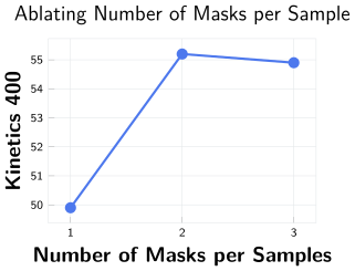
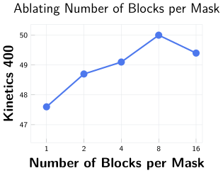
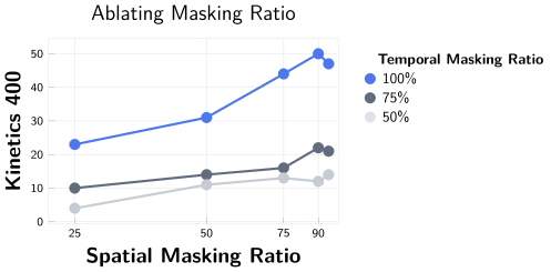
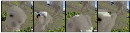
Twenty-six mask ablations show that broad spatial and temporal coverage, several constituent blocks and two complementary masks are useful. Lower coverage creates an easier task that transfers less well in these experiments. The appendix retains both numerical sweeps and visual examples of the masks.