At a glance
Visual imitation policies can reuse familiar environmental factors in unfamiliar combinations, allowing data collection to cover individual values without exhaustively covering their Cartesian product. Simulation and a real fork-placement task favor structured variation, especially the Stair strategy. Real-world composition depends strongly on prior robot data: Stair with BridgeData V2 transfers to new kitchens in 31/40 trials, versus 1/40 for equally sized in-domain data without variation.
I Introduction
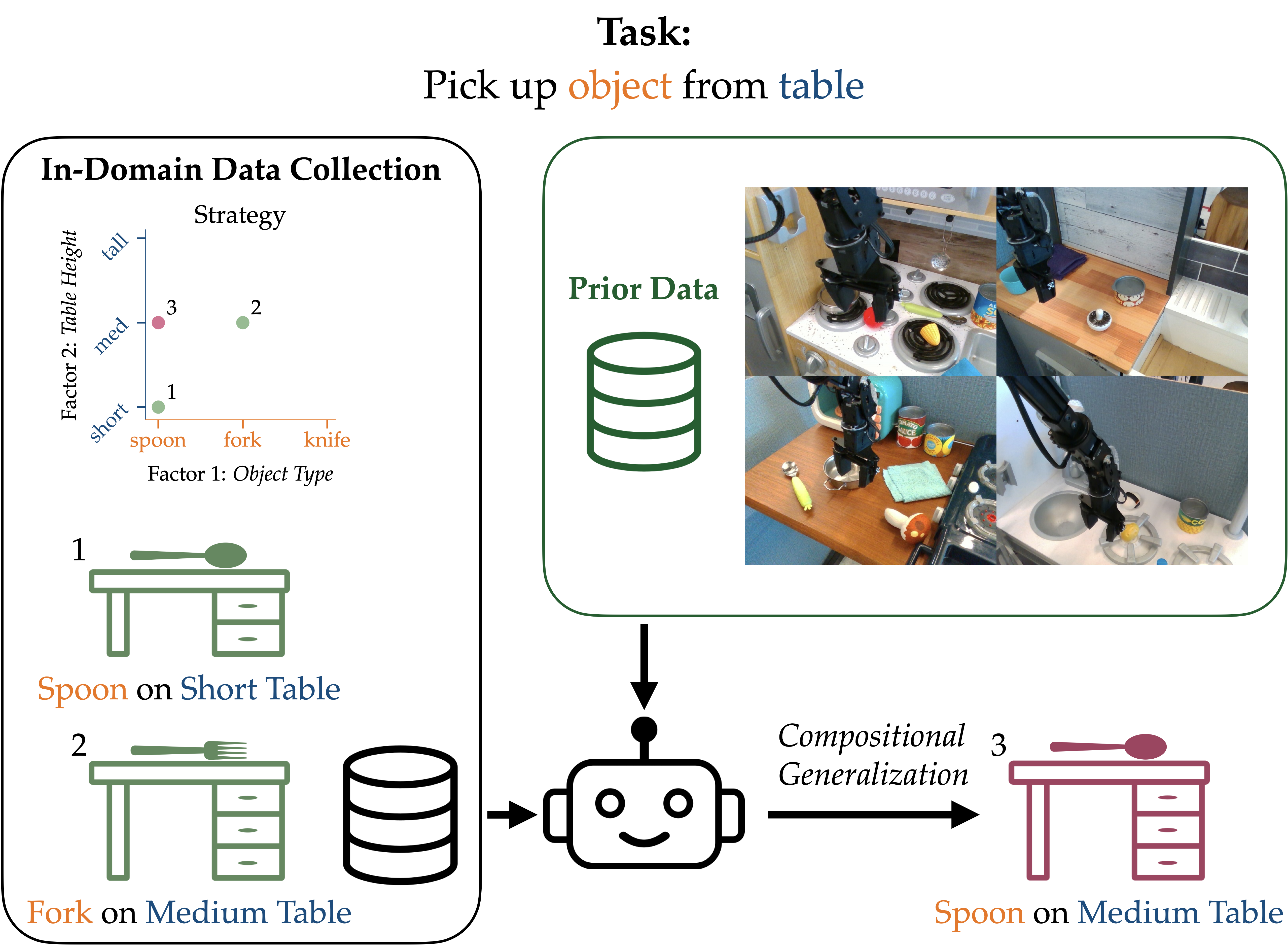
The study treats environmental composition as a data-collection problem. If a policy can combine familiar objects, positions, surfaces, and heights, demonstrators can avoid recording every combination. It compares collection schedules at fixed demonstration budgets and approximately matched numbers of factor changes, then tests when prior robot data supports this generalization.
II Related Work
Previous work emphasizes larger datasets, pretrained visual representations, or semantic composition of skills and instructions. This paper instead varies concrete environmental factors that change images or required motions, and asks how their coverage should guide in-domain demonstration collection. It evaluates existing imitation policies rather than proposing a new compositional architecture. [38], [16], [5].
III Exploiting Compositional Generalization for Efficient Data Collection
The framework separates environmental factors, collection effort, and policy generalization.
III-A Problem Statement
A factor vector specifies environmental conditions and thereby initial-state and goal distributions. Goal-conditioned behavior cloning learns from expert trajectories labeled implicitly by these conditions; evaluation measures the probability of reaching the associated goal across factor combinations.
Equation 1
| (1) |
III-B Objective
With N factors and k values each, exhaustive coverage grows as k to the N, whereas covering every individual value requires only order kN changes. This saving is useful only when the learned policy can compose those values. The experiments therefore measure both overall coverage-based generalization and success specifically on unseen combinations of seen values.
III-C Data Collection Strategies
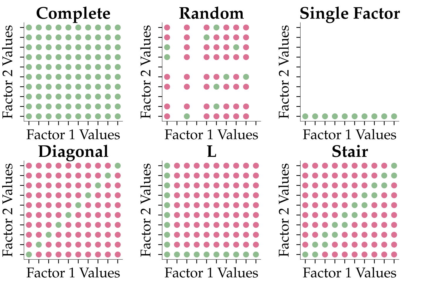
Complete covers every combination; Random resamples combinations; Single Factor changes only one dimension; No Variation keeps the base scene. Diagonal introduces unseen values for all factors together. L varies one factor relative to the base scene. Stair cycles through factors while retaining previous changes, producing more diverse overlapping combinations. Factor-change counts approximate effort and do not model all practical costs of resetting scenes.
III-D Hypotheses
The hypotheses are that structured coverage can beat Random and approach Complete, that Stair benefits from its more varied combinations, and that prior robot data strengthens real-world composition.
IV Simulation Experiments
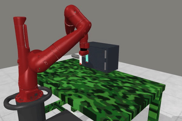
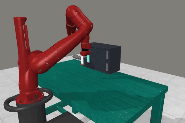
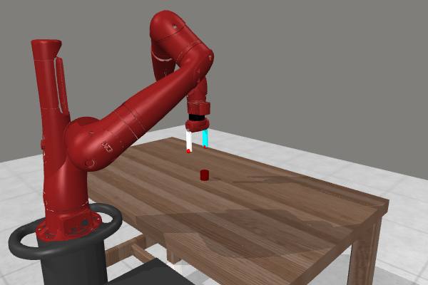
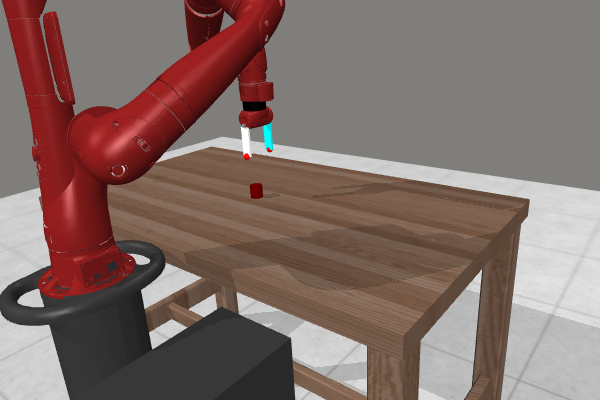
Factor World provides Pick Place and Door Open simulations with controlled environmental variation.
IV-A Evaluation Protocol
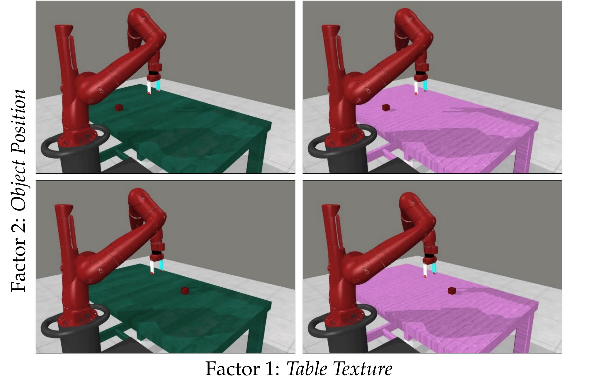
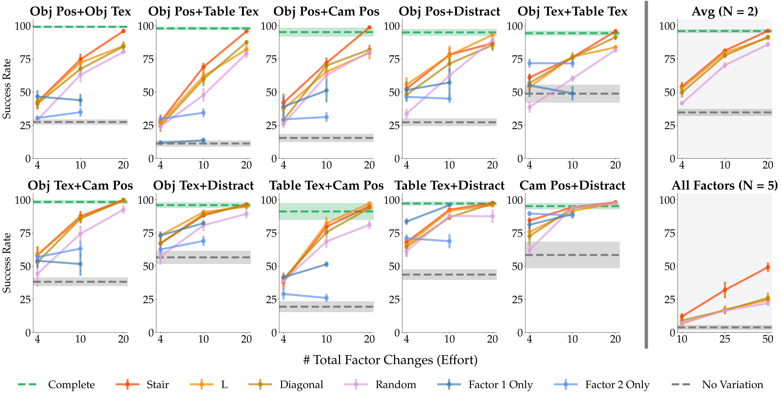
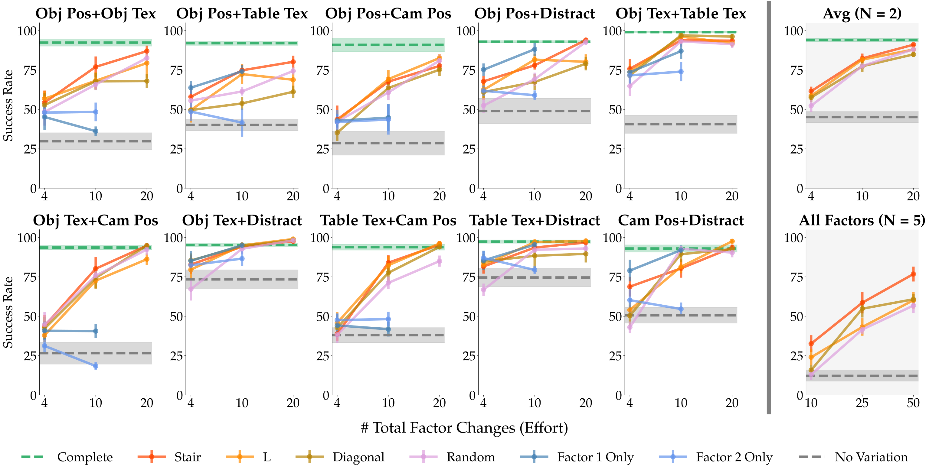
Five factors each have ten values: object texture, table texture, camera position, distractors, and object position. Every factor pair is tested with 100 demonstrations; all five factors use 1,000. Policies are evaluated over 100 episodes and five random seeds. Complete is feasible only for pairs; exhaustive five-factor coverage would require at least 100,000 demonstrations.
IV-B Results
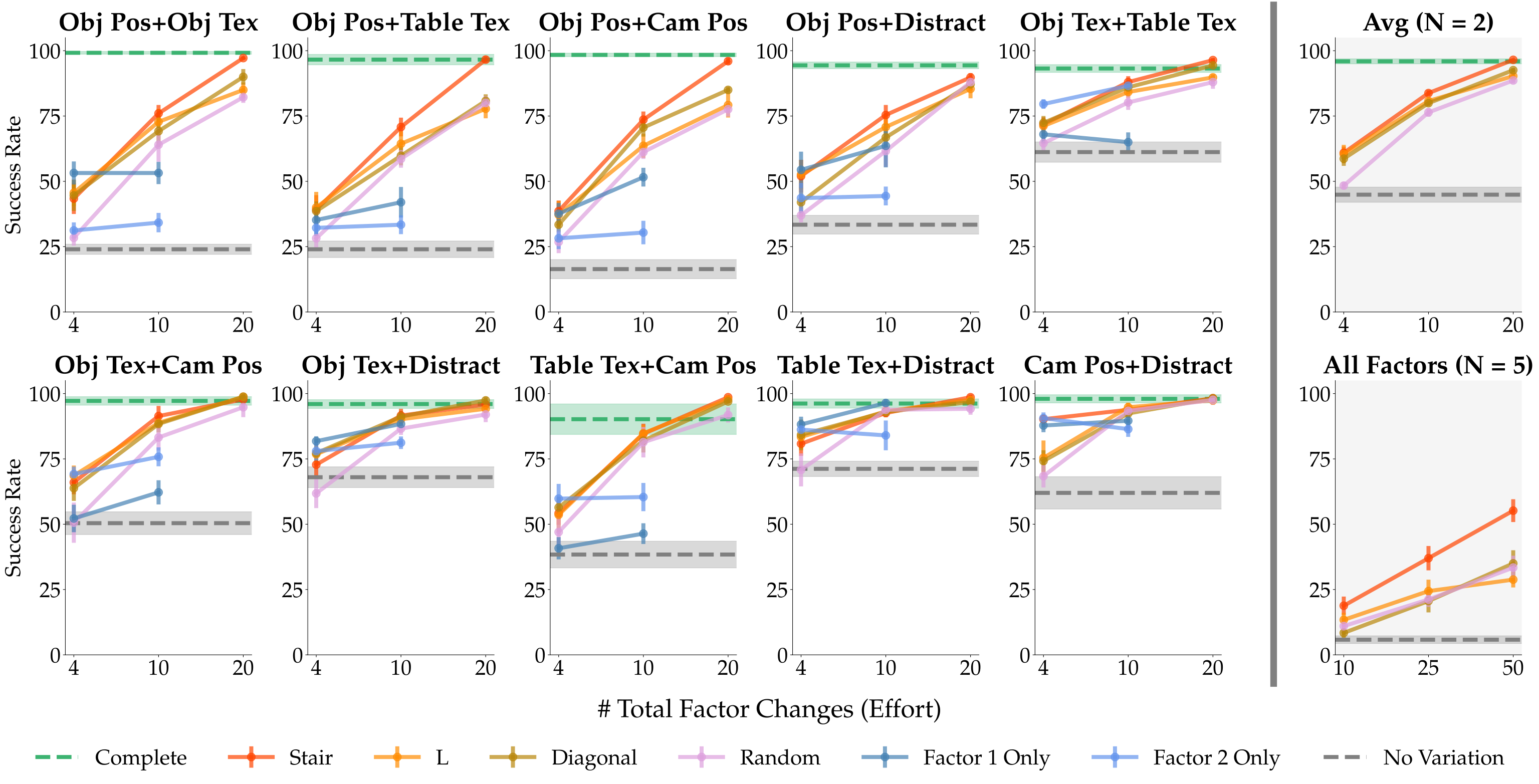
For pairs, Stair, L, and Diagonal generally outperform Random and approach Complete after roughly 20 factor changes rather than 100. With five factors, Stair is the only structured strategy with a substantial advantage over Random. Increasing demonstrations at fixed variation helps Stair most; more examples of an unchanged scene do not solve the generalization problem.
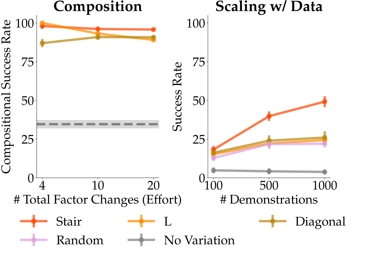
(right) Generalization of strategies with increasing dataset sizes.
V Real Robot Experiments
Real experiments test whether these compositional effects survive visual and physical variability outside simulation.
V-A Evaluation Protocol
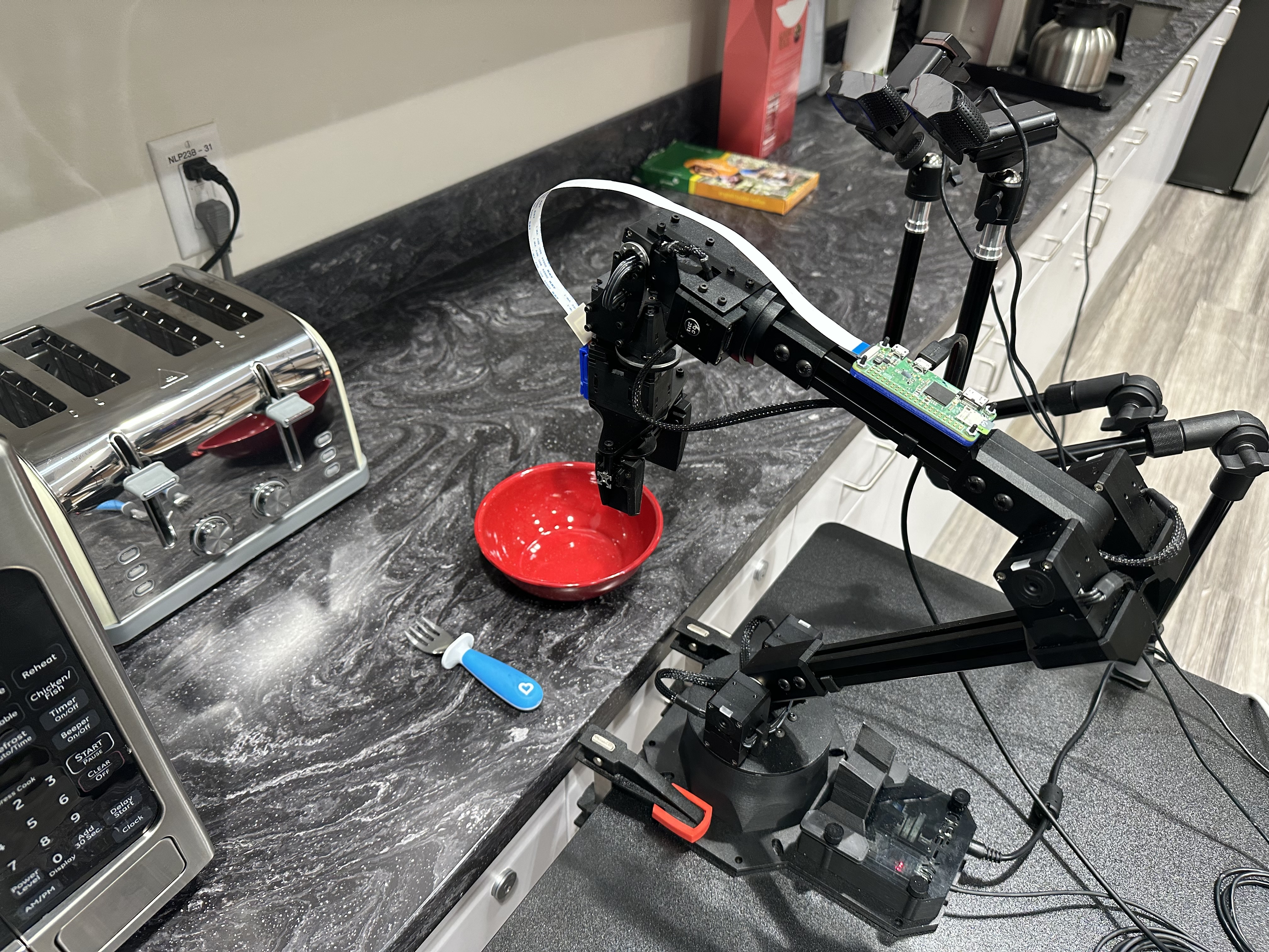
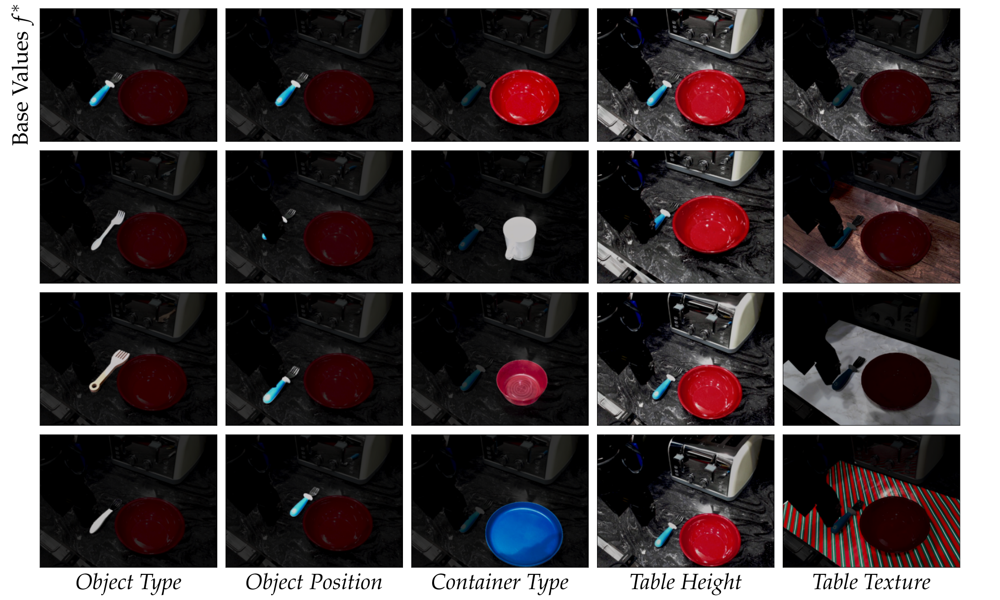
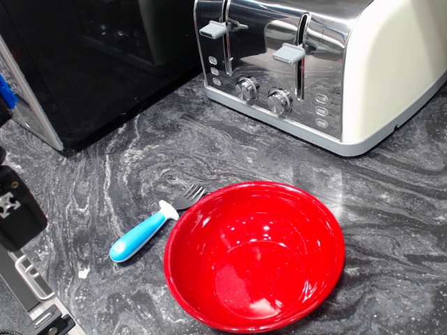
A WidowX 250 arm places a fork into a container. Five primary factors each have four values: fork type and position, container type, table height, and table texture. Stair and L each use 160 demonstrations covering 16 configurations; No Variation uses the same count. Models either train from scratch or pretrain and co-fine-tune with BridgeData V2. [47].
| Data Strategy | L | No Variation | ||||||||||
| Train Method | Bridge | From Scratch | Bridge | |||||||||
|
Object Type |
Container Type |
Table Height |
Table Tex |
Object Type |
Container Type |
Table Height |
Table Tex |
Object Type |
Container Type |
Table Height |
Table Tex | |
| Object Pos | 8/9 | 5/9 | 2/9 | 5/9 | 0/9 | 0/9 | 0/9 | 1/9 | 3/9 | 2/9 | 1/9 | 1/9 |
| Object Type | 8/9 | 8/9 | 8/9 | 5/9 | 5/9 | 4/9 | 4/9 | 3/9 | 2/9 | |||
| Container Type | 5/9 | 6/9 | 4/9 | 6/9 | 2/9 | 3/9 | ||||||
| Table Height | 4/9 | 3/9 | 1/9 | |||||||||
| Overall | 59/90 | 28/90 | 22/90 | |||||||||
V-B Pairwise Composition
Across 90 unseen pairwise combinations, L with BridgeData succeeds in 59, versus 28 from scratch and 22 for No Variation with BridgeData. Physically interacting changes, such as object position and table height, remain difficult. Frozen R3M and VC-1 encoders perform poorly in the tested 27-case subset; these results concern the reported diffusion-policy implementations, not every possible use of pretrained representations.
| Data Strategy | L | No Variation | |||||
| Train Method | Bridge | R3M | VC-1 | From Scratch | Bridge | R3M | VC-1 |
|
Object Type + Table Tex |
8/9 | 1/9 | 0/9 | 4/9 | 2/9 | 0/9 | 0/9 |
|
Object Pos + Table Tex |
5/9 | 0/9 | 0/9 | 1/9 | 1/9 | 0/9 | 0/9 |
|
Object Pos + Table Height |
2/9 | 1/9 | 0/9 | 0/9 | 1/9 | 0/9 | 0/9 |
| Overall | 15/27 | 2/27 | 0/27 | 5/27 | 4/27 | 0/27 | 0/27 |
| Data Strategy | Stair | L | No Variation | ||||||
| Train Method |
Bridge (Co-FT) |
Bridge (FT) |
From Scratch |
Bridge (Co-FT) |
Bridge (FT) |
From Scratch |
Bridge (Co-FT) |
Bridge (FT) | |
|
No Further Changes |
CompKitch | 4/5 | 4/5 | 0/5 | 5/5 | 0/5 | 0/5 | 0/5 | 0/5 |
| TileKitch | 5/5 | 2/5 | 0/5 | 5/5 | 5/5 | 3/5 | 0/5 | 0/5 | |
|
Fork Down + Blue Plate |
CompKitch | 4/5 | 4/5 | 0/5 | 3/5 | 0/5 | 0/5 | 1/5 | 0/5 |
| TileKitch | 4/5 | 3/5 | 0/5 | 3/5 | 5/5 | 5/5 | 0/5 | 0/5 | |
|
Wooden Fork + Pink Bowl |
CompKitch | 3/5 | 5/5 | 0/5 | 2/5 | 0/5 | 0/5 | 0/5 | 0/5 |
| TileKitch | 4/5 | 3/5 | 0/5 | 3/5 | 5/5 | 2/5 | 0/5 | 0/5 | |
|
Plastic Fork + Higher Table |
CompKitch | 4/5 | 0/5 | 0/5 | 1/5 | 0/5 | 0/5 | 0/5 | 0/5 |
| TileKitch | 3/5 | 0/5 | 0/5 | 2/5 | 0/5 | 1/5 | 0/5 | 0/5 | |
| Overall | CompKitch | 15/20 | 13/20 | 0/20 | 11/20 | 0/20 | 0/20 | 1/20 | 0/20 |
| TileKitch | 16/20 | 8/20 | 0/20 | 13/20 | 15/20 | 11/20 | 0/20 | 0/20 | |
| Combined | 31/40 | 21/40 | 0/40 | 24/40 | 15/40 | 11/40 | 1/40 | 0/40 | |
V-C Out-Of-Domain Transfer
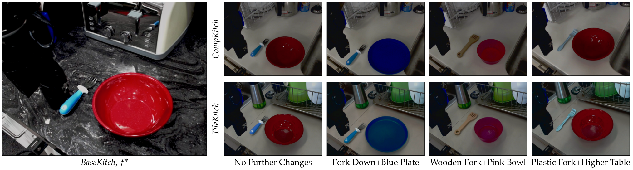
Two new kitchens introduce unseen factor values and additional uncontrolled shifts. Across 40 trials, co-fine-tuned Stair scores 31/40 and L 24/40, versus 1/40 for No Variation. Fine-tuning without retaining prior data falls to 21/40 and 15/40. From-scratch Stair scores 0/40 and L 11/40. Prior data and varied in-domain demonstrations both contribute.
V-D Additional Experiments
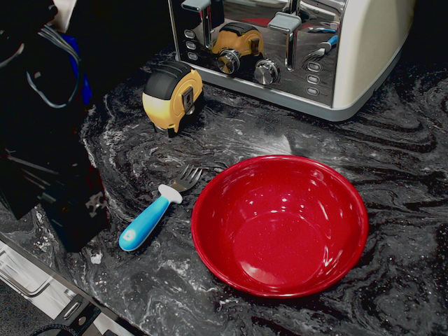
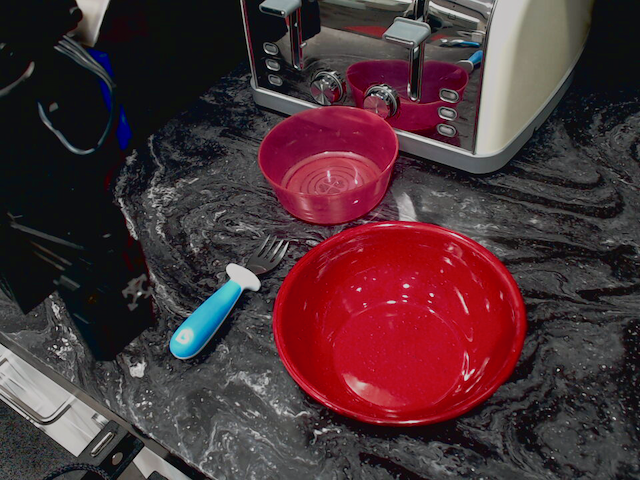
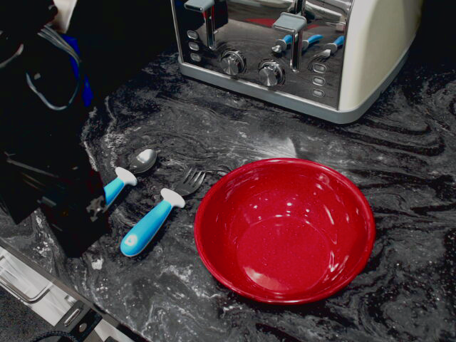
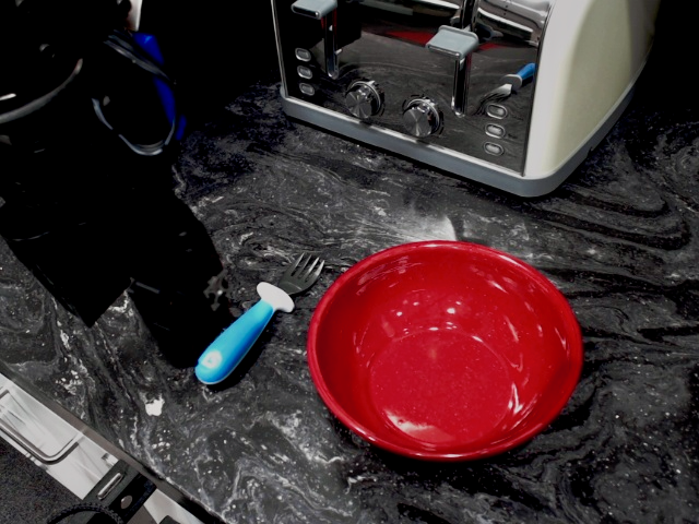
Held-out distractors can reduce robustness when structured datasets train from scratch; prior data restores 15/15 successes in this test. A separate camera/texture composition experiment reaches 10/10 with both complementary datasets and BridgeData, versus 1/10 or 6/10 using either dataset alone. None of the corresponding from-scratch models succeeds.
| Data Strategy | Stair | L | No Variation | |||
| Train Method | Bridge |
From Scratch |
Bridge |
From Scratch |
Bridge |
From Scratch |
| Tape Measure | 5/5 | 1/5 | 5/5 | 5/5 | 5/5 | 5/5 |
| Pink Bowl | 5/5 | 3/5 | 5/5 | 4/5 | 5/5 | 5/5 |
| Spoon | 5/5 | 5/5 | 5/5 | 0/5 | 5/5 | 4/5 |
| Overall | 15/15 | 9/15 | 15/15 | 9/15 | 15/15 | 15/15 |
| Train Method | Bridge | From Scratch |
| No Camera Position | 1/10 | 0/10 |
| No Table Texture | 6/10 | 0/10 |
| Both | 10/10 | 0/10 |
VI Discussion
The findings motivate systematic variation without establishing universal compositional guarantees.
VI-A Summary
Stair is generally strongest in the reported comparisons, while L can be operationally convenient when factors are easier to vary separately. Prior robot data supports both composition and robustness to unmodeled changes. Physical interactions may still warrant denser coverage than purely visual variation.
VI-B Limitations and Future Work
Real experiments center on one robot, one main task, and one prior dataset. A preliminary attempt to compose a new removal task with existing factor variation fails. The results do not establish how to collect an optimal large-scale prior dataset, and factor interactions, different architectures, and other learning methods remain open questions.
Acknowledgments
The authors acknowledge DARPA, ONR, NSF, Toyota Research Institute, and colleagues who supported the experiments and robot setup.
Appendix A Data Collection Strategies
The appendix specifies the proposed collection schedules.
A-A Pseudocode
The three retained algorithms distinguish simultaneous unseen-value changes (Diagonal), one-factor deviations from the base scene (L), and cyclic changes that retain previous settings (Stair).
Appendix B Simulation Experiments
The simulation appendix reports additional results, sampling choices, augmentation, and effort accounting.
B-A Door Open Results
Door Open broadly reproduces the Pick Place pattern: strong pairwise composition and a larger Stair advantage when all five factors vary.
B-B Factors
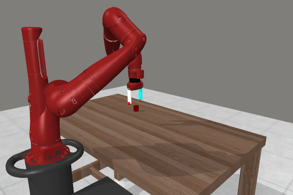
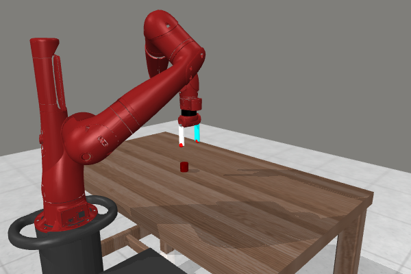
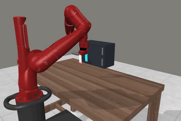
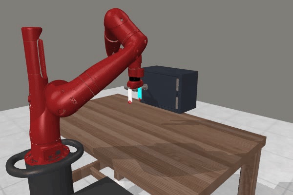
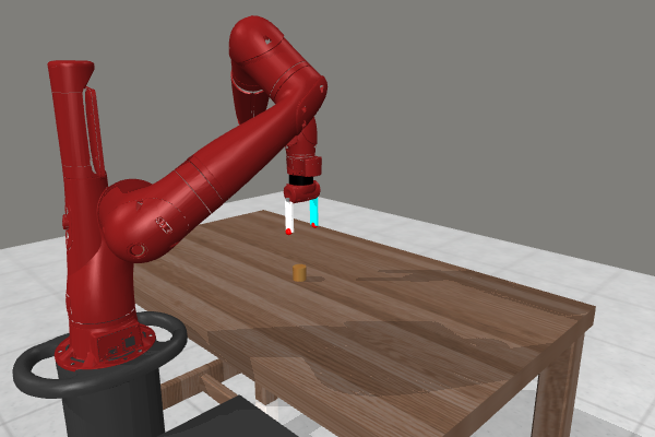
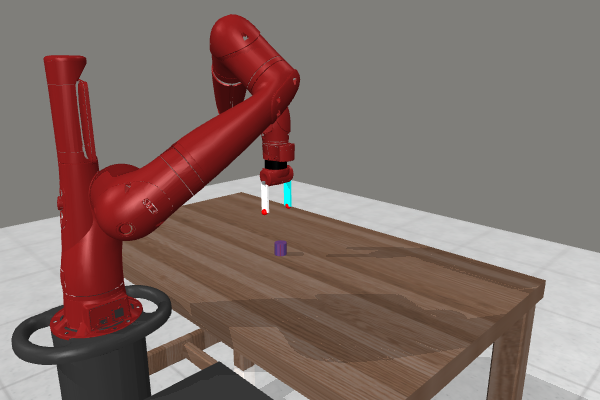
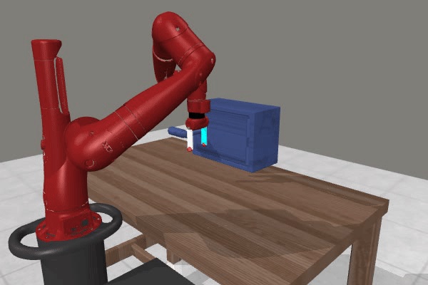
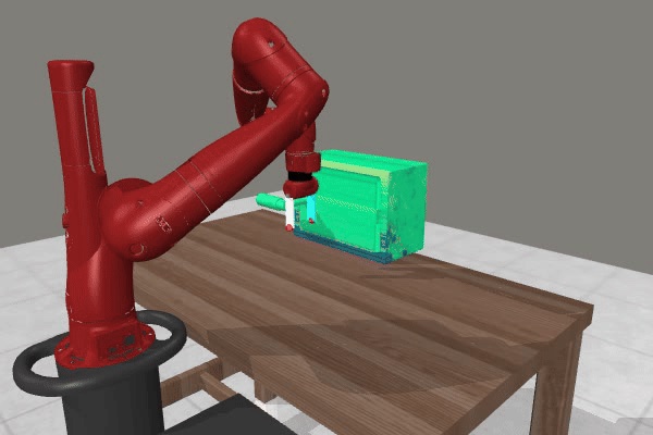
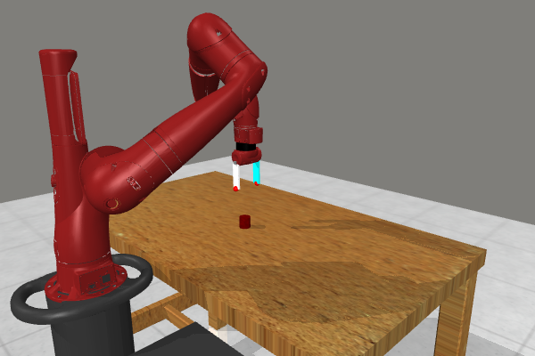
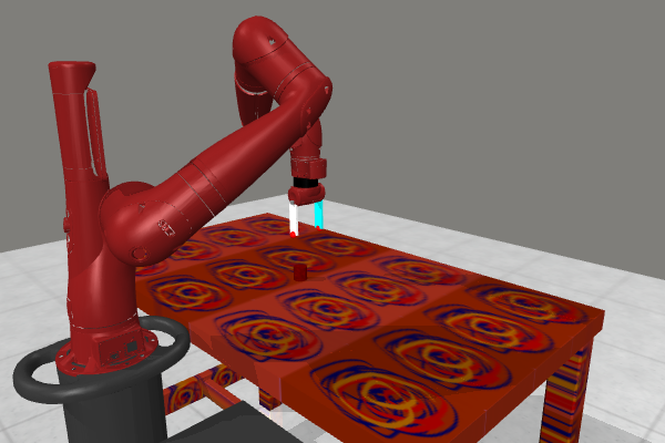
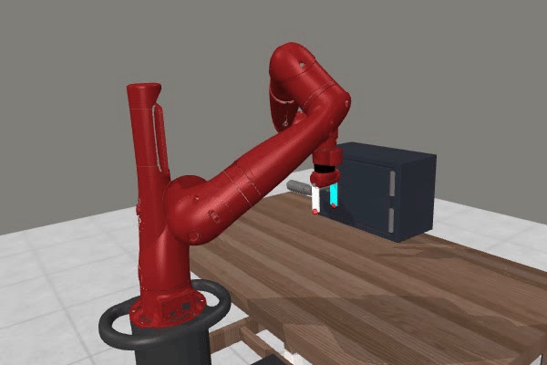
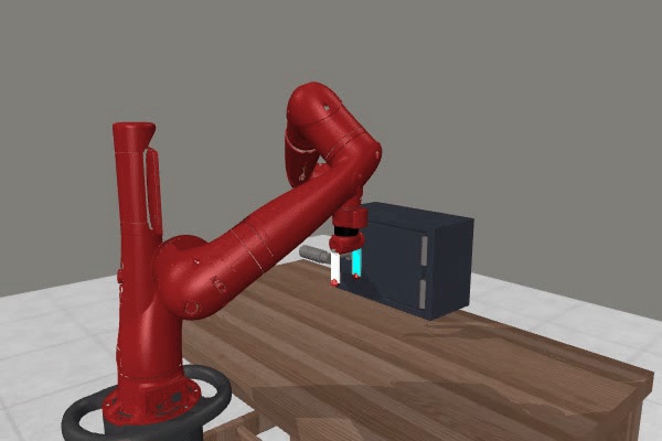
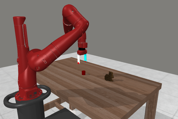
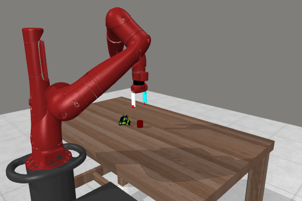
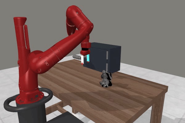
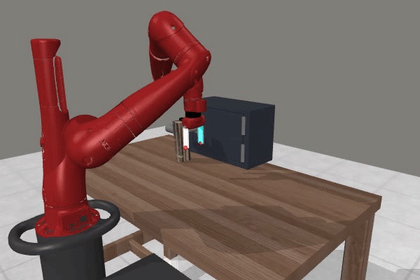
Textures and distractors are sampled from Factor World training values; positions and camera poses use bounded perturbations. Samples must remain solvable by the scripted expert. Each seed resamples the ten allowed values, and Pick Place retains small per-episode position noise.
B-C Training
Simulation policies use two 84×84 RGB views and proprioception, with end-effector displacement and gripper actions. Random-shift augmentation is always enabled. These single-task models omit goal conditioning.
B-D Color Jitter Augmentation
Adding color jitter slightly improves overall performance while preserving the main ranking among collection strategies.
B-E Accounting for Factor Value Similarity
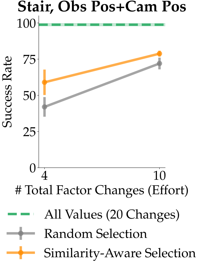
For object and camera positions, selecting representative values by k-medoids improves Stair over random value selection at the same change budget. It still trails observing all values. Extending this approach to objects or textures requires useful similarity measures.
B-F Computing Factor Changes
Effort counts include initial factor setup. Stair, L, and Single Factor count one change per subsequent configuration; Diagonal and Random count one per factor. This can underestimate L resets and overestimate Random when sampled values repeat. Demonstrations are divided across the configurations allowed by each budget.
Appendix C Real Robot Experiments
The real-world appendix retains extra kitchen views, model details, and factor analyses.
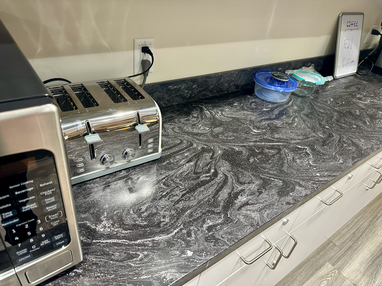
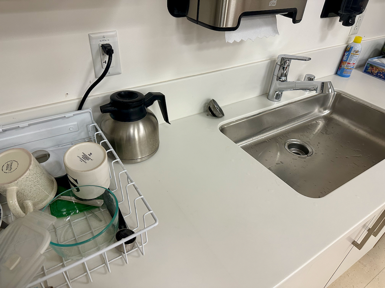
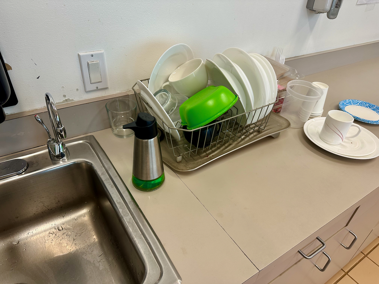
C-A Robot Platform
Experiments use third-person webcams. A wrist camera helped some from-scratch policies but impaired transfer from BridgeData, which contains relatively little wrist-camera coverage; it is omitted from the reported experiments.
C-B Evaluation Protocol
One experienced operator collects demonstrations with a Quest 2 headset. Relative table height is changed by adjusting the robot platform. Stair follows a fixed cycle through fork position, fork type, container type, table height, and texture.
C-C Training
The ResNet-34 diffusion policy uses two 128×128 image observations plus a goal image and predicts four actions, usually executing only the first. BridgeData pretraining runs for two million steps; fine-tuning uses 300,000. Co-fine-tuning mixes 75% in-domain and 25% prior data. Additional-factor results are retained in Table VI.
| Data Strategy | L | |||||||||
| Train Method | Bridge | From Scratch | ||||||||
|
Object Pos |
Object Type |
Container Type |
Table Height |
Table Tex |
Object Pos |
Object Type |
Container Type |
Table Height |
Table Tex | |
| Object/Container Pos | N/A | 7/9 | 6/9 | 2/9 | 6/9 | N/A | 5/9 | 2/9 | 0/9 | 3/9 |
| Object Orientation | 2/9 | 5/9 | 5/9 | 1/9 | 3/9 | 0/9 | 2/9 | 3/9 | 0/9 | 1/9 |
| Overall | 36/81 | 16/81 | ||||||||
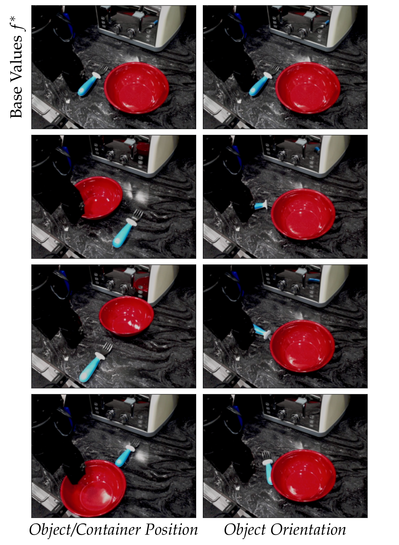
C-D Pairwise Composition for Additional Factors
Adding joint fork/container positions and fork orientations yields 36/81 compositional successes with prior data versus 16/81 without it. Orientation requires separate training with half the in-domain batch allocated to that factor and remains especially difficult.
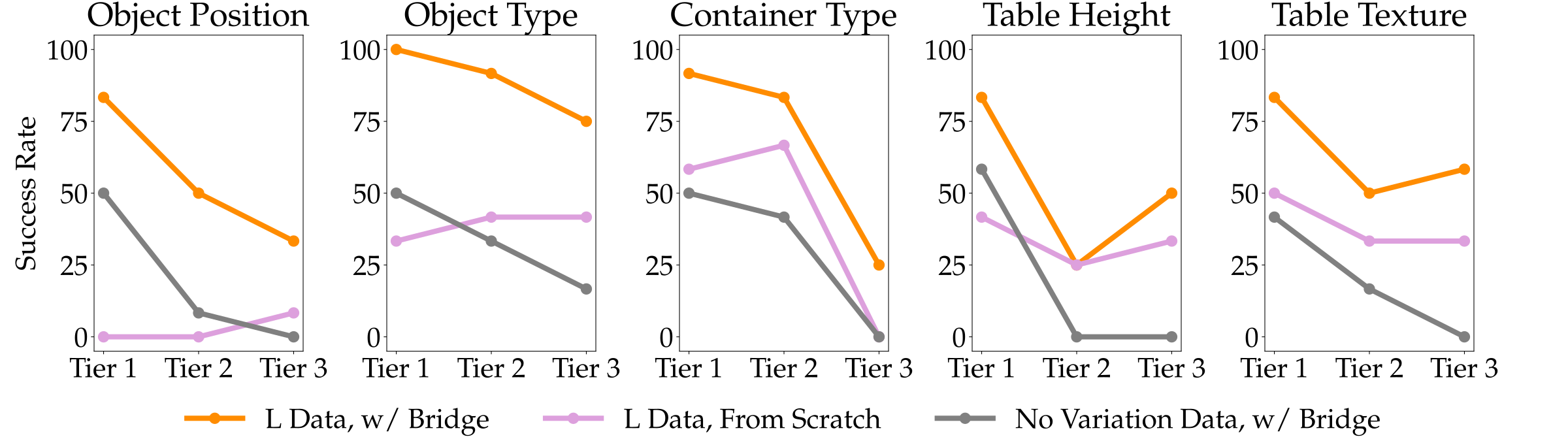
C-E Factor Similarity Analysis
Factor values are ranked by a No Variation policy’s success as a proxy for similarity to the base scene. More dissimilar values generally compose less well, although the ranking also reflects intrinsic task difficulty and trends are not strictly monotonic.
| Factor | Tier 1 | Tier 2 | Tier 3 |
| Object Pos | Down (3) | Up (4) | Left (2) |
| Object Type | Wooden (3) | Gray (4) | Plastic (2) |
| Container Type | Blue Plate (4) | Pink Bowl (3) | White Cup (2) |
| Table Height | Higher 5cm (2) | Lower 5cm (3) | Lower 8cm (4) |
| Table Tex | Brown Wood (2) | Gift Wrap (4) | White Marble (3) |
C-F R3M
R3M features use ResNet-50, dataset normalization, a diffusion head without goal conditioning, 500,000 training steps, and execution of all four predicted actions to reduce jitter. These changes make the frozen-encoder comparison distinct from the end-to-end setup.
C-G VC-1
VC-1 follows the R3M training and evaluation procedure, substituting its ViT-L visual encoder.