At a glance
SNDS learns an autonomous velocity policy and a convex Lyapunov candidate together. A projection constrains the policy’s energy change, while a short-horizon trajectory loss improves imitation beyond pointwise velocity fitting. Handwriting experiments and a Kinova arm demonstrate recovery and accurate reproduction with few demonstrations. The paper claims global asymptotic stability; the displayed projection and numerical implementation require care when interpreting that claim.
I Introduction
Behavior cloning can reproduce familiar demonstrations yet behave unpredictably after a perturbation. Stable dynamical-system policies aim to converge to the same target from unfamiliar states, but restrictive model classes and expensive fitting can limit their accuracy and scalability. SNDS combines a neural policy, a learned convex potential, and differentiable training to address those limitations.
The contribution is a policy architecture plus a trajectory-alignment objective, evaluated on planar handwriting and pose trajectories. Convergence to a target should be distinguished from collision avoidance or compliance with robot limits, which this work does not enforce.
II Background
The policy is an autonomous differential equation whose output is a state derivative. Training demonstrations share one terminal state.
II-A Preliminaries
A DS maps the current state to velocity without explicit time dependence. Lyapunov analysis relates convergence to a positive-definite potential that decreases along trajectories. An ICNN supplies a convex function with architectural weight and activation restrictions; this potential is learned alongside the motion field.
Equations
II-B Problem statement
Training data contain sampled position–velocity pairs from several demonstrations, all ending at the same target with zero terminal velocity. The objective is a deterministic state-to-derivative mapping that reproduces these motions and generalizes away from them. Rollouts use forward Euler integration, so the simulation step size also affects the realized trajectory.
Equations 1–2
| (1) |
| (2) |
III Methodology
The method builds a projected neural vector field, analyzes its Lyapunov behavior, and trains it using velocity and short-horizon position errors.
III-A Dynamical system policy formulation
An unrestricted feedforward network proposes a velocity. A second network defines the potential by subtracting its target value and adding a positive quadratic term. Equation (4) removes the component of the proposed velocity that violates the prescribed Lyapunov half-space. Automatic differentiation permits joint optimization.
The paper uses ReLU for this projection and relaxes an earlier exponentially stable formulation. The exact displayed equations are preserved because the distinction between nonincreasing and strictly decreasing potential matters to the subsequent guarantee.
Equations 3–4
| (3) |
| (4) |
III-B Global asymptotic stability guarantees
Proposition 1 states that the constructed policy is globally asymptotically stable. Its contradiction argument assumes a positive-definite potential and a uniformly negative derivative on a compact set away from the target, then integrates that decrease until it contradicts nonnegativity.
Reading note: with the stated ReLU, equation (4) gives dV/dt = min(∇V·π̂, 0) wherever its denominator is nonzero. This ensures a nonpositive derivative, but does not by itself establish the strict decrease used in the proof. Convexity and subtracting a target value likewise do not alone make that target the minimum of an arbitrary convex network. The convergence claim therefore needs these additional conditions to hold; the empirical recovery results remain separate evidence.
Equations
III-C SRVF training loss
Velocity MSE can be small even when integration accumulates substantial position error. The proposed objective combines velocity fitting with discounted short-horizon Euler position errors and SRVF-based trajectory features. A short horizon keeps gradients and memory manageable; the experiments use two steps with weights γᵢ = 2⁻ⁱ. The retained equations give the precise feature transform and loss.
Equations 5–6
| (5) |
| (6) |
IV Experiments
Evaluation uses LASA handwriting and a more complex Messy Snake dataset. The latter also supplies the trajectory for simulation and hardware deployment.
IV-A Evaluation
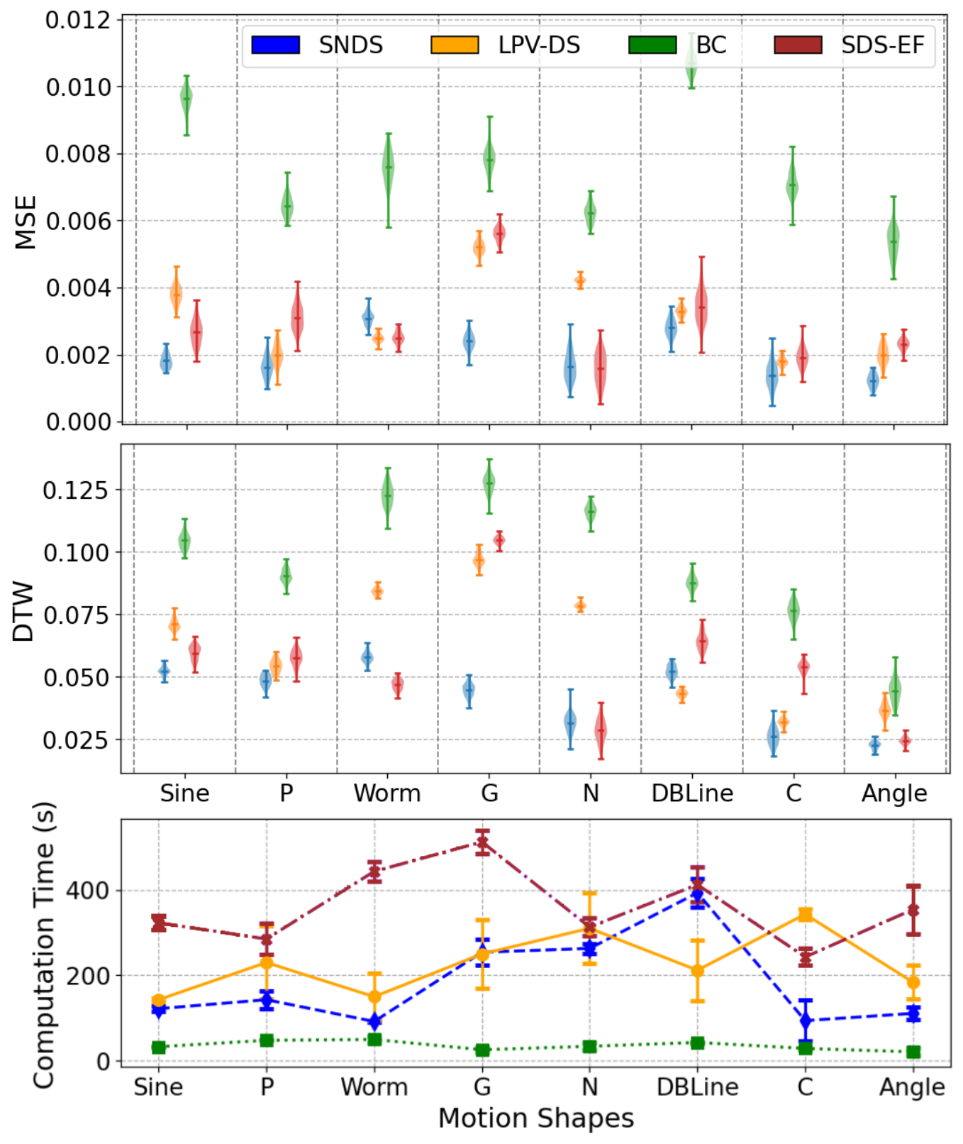
Baselines are ordinary behavior cloning, LPV-DS, and SDS-EF. The experiments use an 80/20 train/test split and ten random seeds. MSE measures velocity prediction, while DTW compares complete generated and demonstrated trajectories; these metrics capture different failure modes. The figures also report learning time.
Equations 7–8
| (7) |
| (8) |
IV-B Handwriting dataset policies
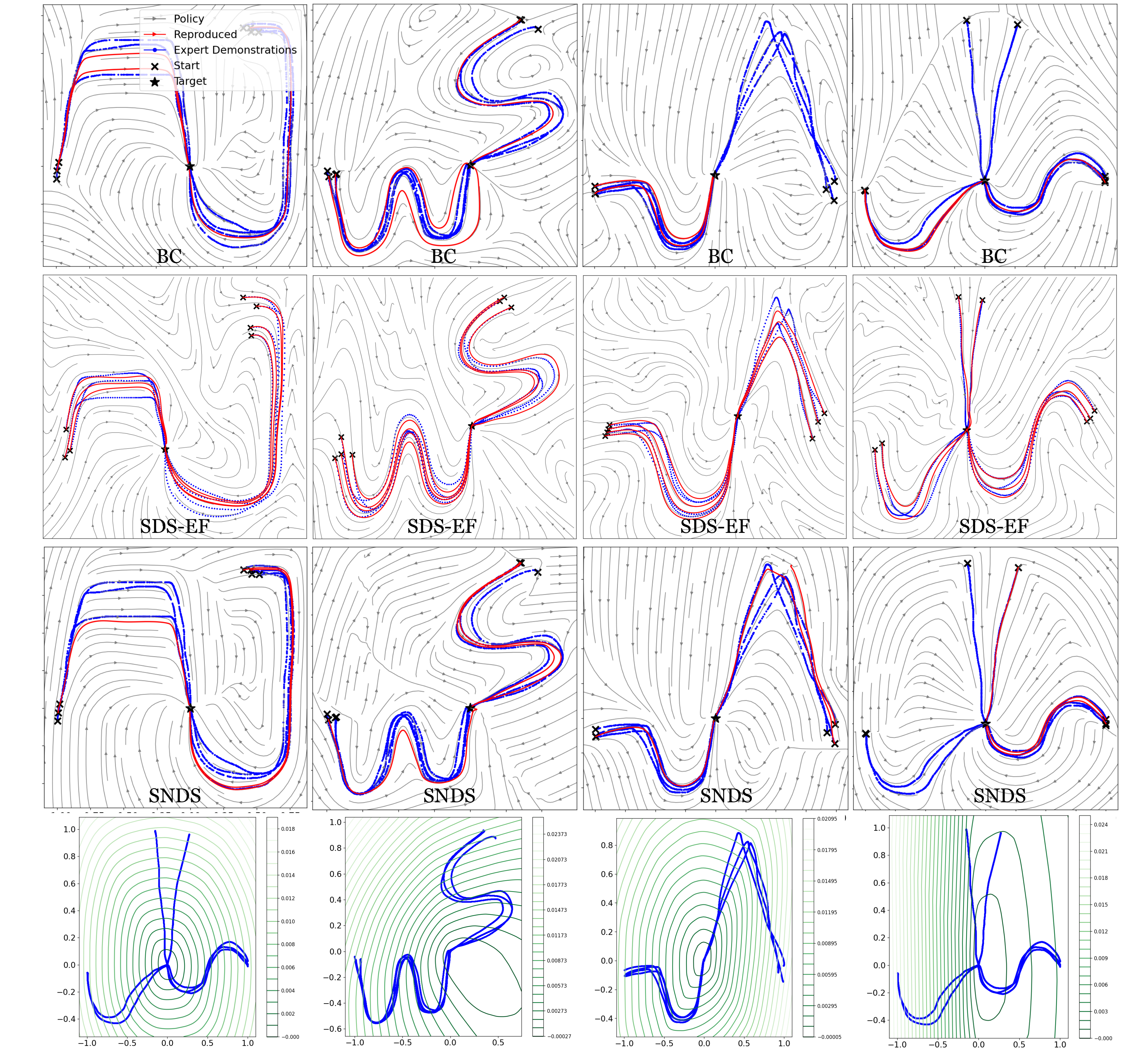
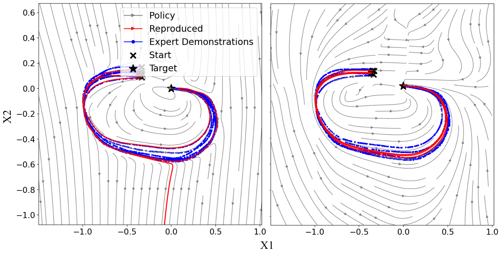
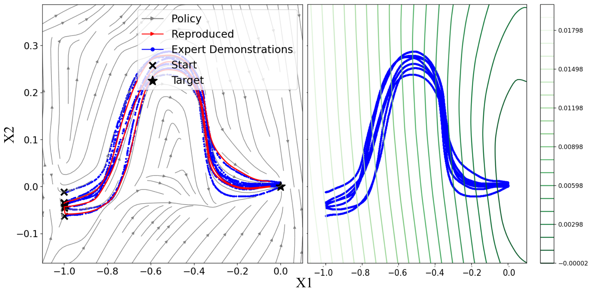
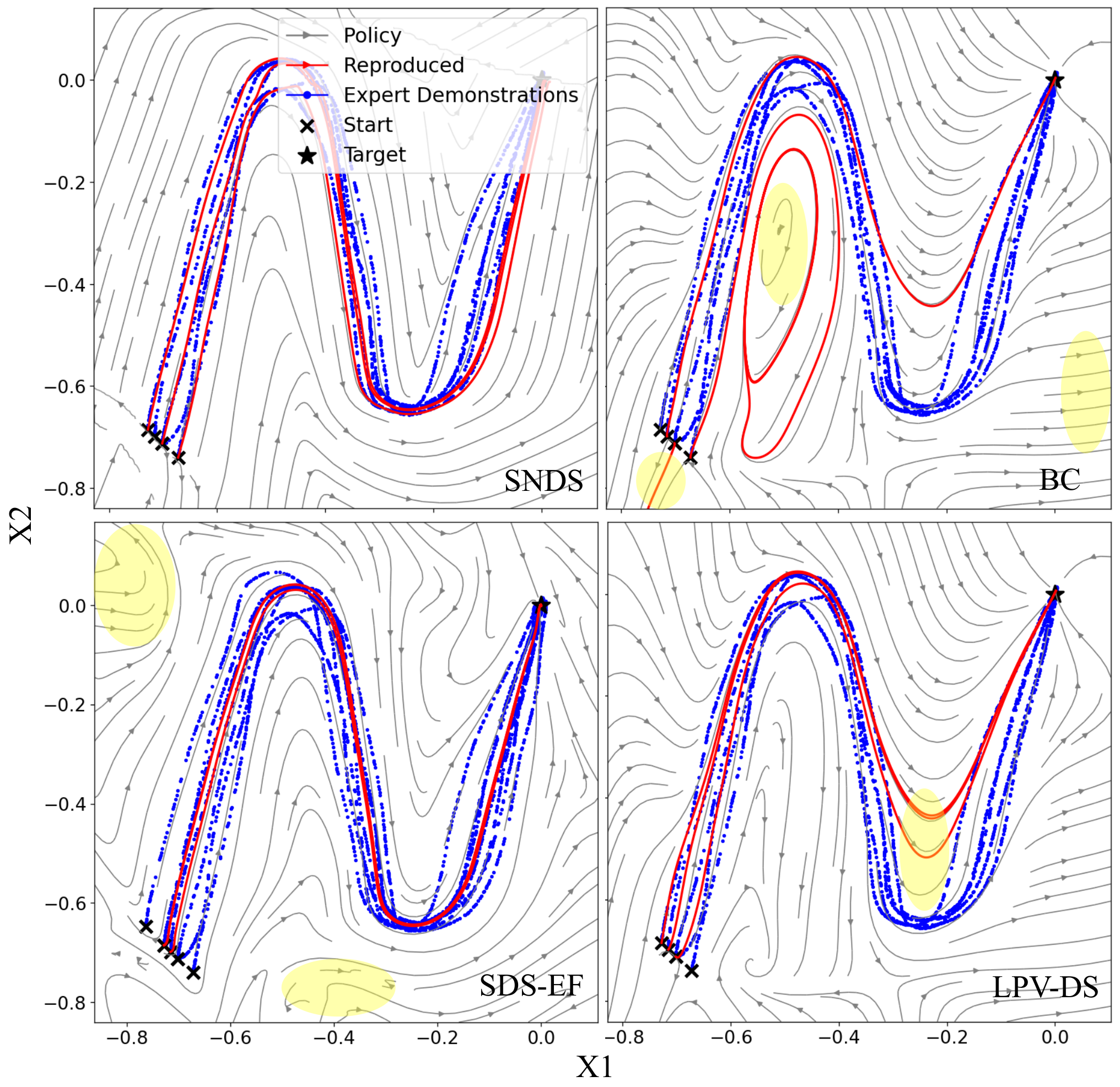
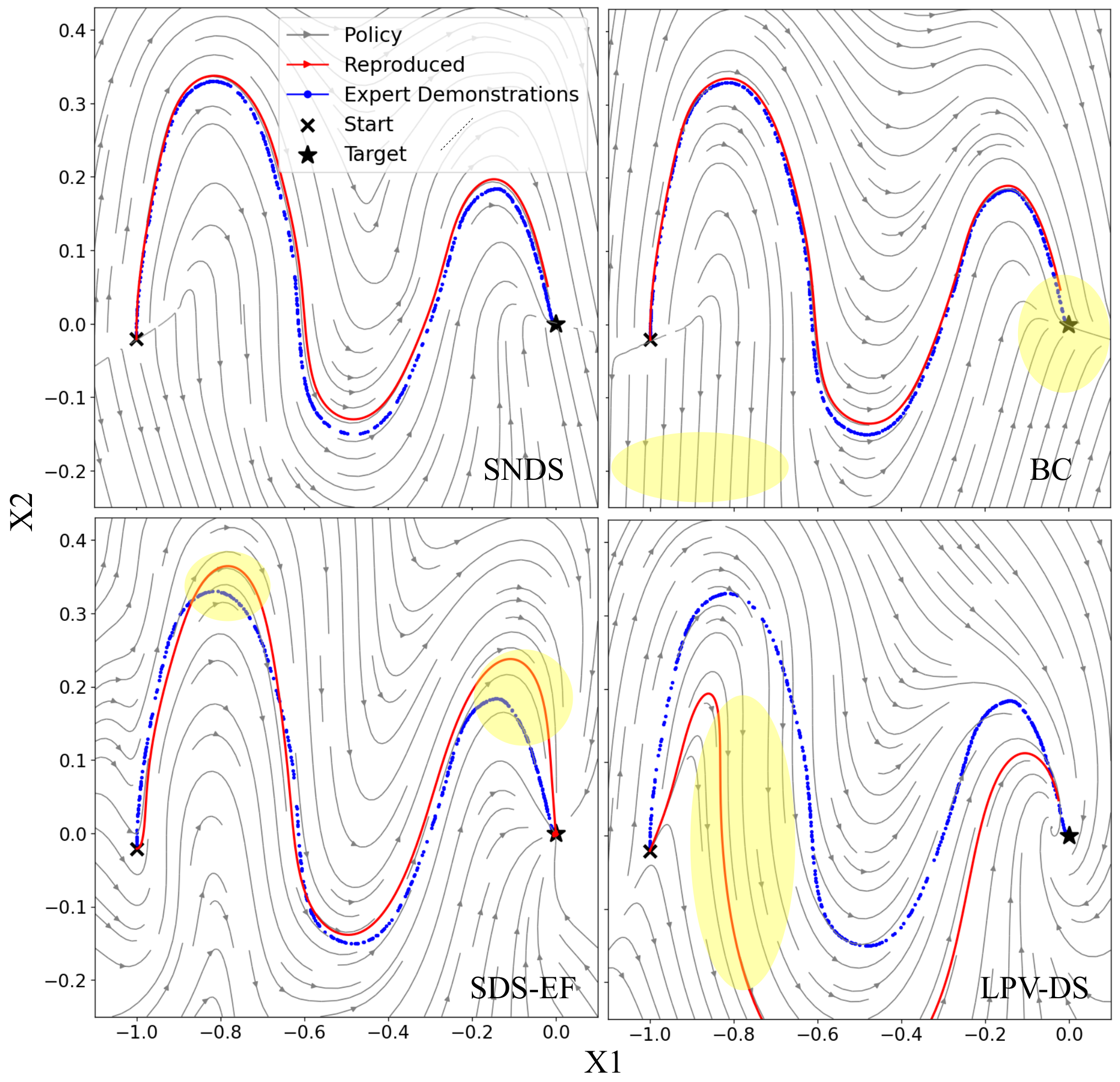
SNDS generally provides favorable imitation error and training time on the selected motions, though it does not win every case. Streamlines and perturbed rollouts illustrate recovery outside the demonstrated region. A single-demonstration Sine experiment tests data efficiency against mixture-model and flow-based policies. These comparisons concern the tested implementations and motions, not all possible models in each family.
IV-C SE(3) policy training
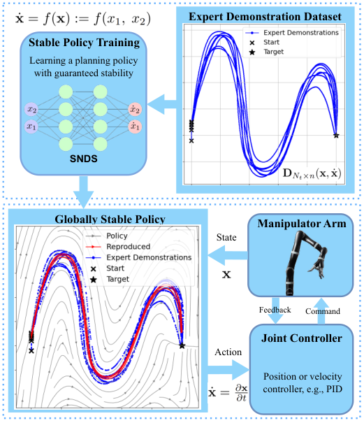
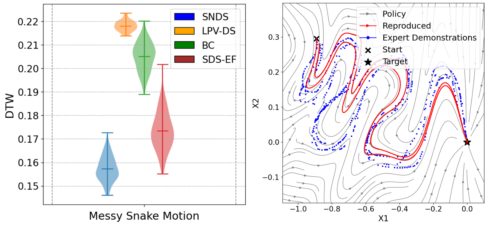
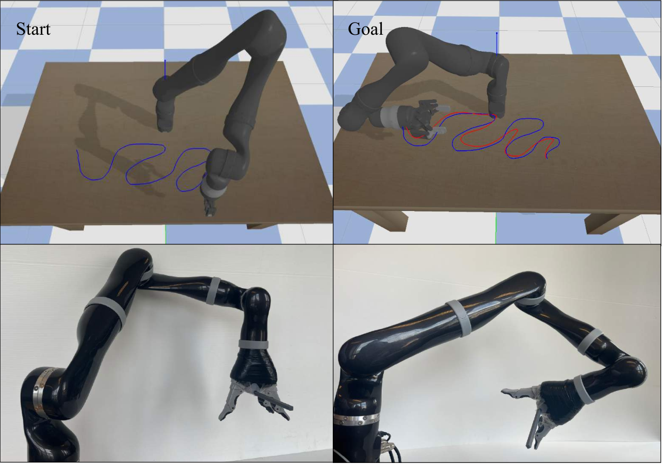
The state is extended to position and orientation for pose imitation. The orientation demonstrations are synthetic additions to translational data. The authors evaluate Sine, G, and Messy Snake motions, deploy the learned field in PyBullet, and transfer it to a Kinova Jaco2 arm. The robot reproduces the demonstrated pattern and recovers in the shown trials. This does not establish global guarantees for every orientation representation or low-level robot controller.
V Discussion
The architecture offers expressive, efficiently trained policies with a learned stability-related structure. Remaining practical gaps include obstacles, joint and torque limits, and physically infeasible generated paths. The authors propose barrier constraints and more flexible Lyapunov representations as future extensions.
VI Conclusion
Joint policy–potential learning and a short-horizon imitation objective produce promising stable-looking rollouts in simulation and on hardware. The method’s formal claims should be read with the conditions discussed above, and kept separate from the demonstrated task performance.
VII Reproducability
The policy network has widths 2–256–256–128–128–2 with Leaky ReLU activations; the ICNN has widths 2–128–128–128–1 with the specified convex activations. The loss uses a two-step horizon. The selected LASA motions come from a dataset with seven demonstrations per motion; Messy Snake has three demonstrations, with one used for the robot experiment.
The timing comparison restricts computation to a single CPU, while the broader implementation reports an RTX 4050 machine. Architecture, data, and executable experiments are available in the authors’ repository.
Acknowledgment
Anya Forestell is acknowledged for hardware support.
Appendix
The appendix explains trajectory differentiation, practical numerical choices, and additional multimodal handwriting experiments.
VII-A Efficient trajectory generation
Short explicit Euler rollouts are the chosen differentiable training procedure. The appendix also discusses implicit differentiation as a memory-conscious alternative, but reports that explicit steps are faster for the small horizons used here. Long-horizon memory advantages are not an evaluated contribution of this implementation.
Equation
VII-B Smoothness and numerical stability
ReLU makes the projection nonsmooth, and a near-zero potential gradient makes its denominator numerically problematic. Suggested remedies include smoother activations, denominator regularization, gradient clipping, and a smoother or Lipschitz-bounded potential network. These changes modify the exact projected field, so the displayed continuous-time argument cannot automatically certify every regularized implementation or Euler step size.
VII-C Additional experiments
Additional handwriting experiments include multiple approach directions toward a shared equilibrium. Figure 9 compares the resulting SNDS, SDS-EF, and behavior-cloning vector fields and shows the learned potential.