At a glance
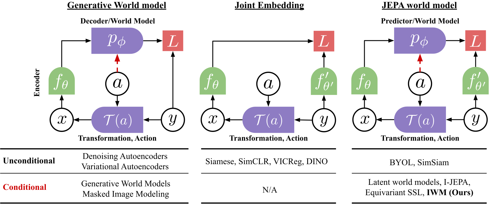
Intuition. Given a picture and the instruction “increase its brightness,” a useful predictor should change the representation in the corresponding way. If it simply removes all brightness information, it cannot perform that instruction. Image World Models extend JEPA beyond filling masked regions by conditioning predictions on image transformations.
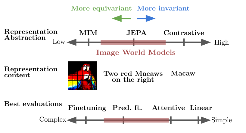
The paper distinguishes keeping information about a transformation from becoming invariant to it. Conditioning, sufficiently difficult transformations and adequate predictor capacity determine the observed behavior. A central downstream result is that the pretrained predictor can be adapted for recognition instead of always being discarded after pretraining.
1 Introduction
Self-supervised image transformations can be interpreted as actions inside a small world model. The encoder represents an image and the predictor models what a specified transformation does to that representation. This does not mean the system has learned physical dynamics from static images. It tests whether transformation modeling learns useful visual features and whether the predictor itself can later help solve classification or segmentation tasks.
2 Related works
2.1 Augmentation invariant Self-Supervised Learning
Augmentation-invariant learning makes related image views share a representation. That can improve recognition by suppressing irrelevant details, but may also remove information useful for another task. Different contrastive and noncontrastive objectives provide different protections against a constant representation.
2.2 World modeling in visual representation learning
Masked image modeling, equivariant representation learning and generative prediction can all be viewed as learning effects of transformations. IWM emphasizes two differences: explicitly condition the latent predictor on what changed, and investigate reusing that predictor downstream rather than evaluating only the encoder.
3 Method
The method constructs source and target views, including masked source patches and different photometric transformations. An encoder represents the source; a momentum-updated target encoder supplies the training target. The predictor receives both the source representation and transformation information, then predicts target patch features. The paper calls a predictor “equivariant” when it can apply the controlled change. Some transformations are destructive rather than invertible group actions, so this term describes the tested predictive behavior rather than a universal mathematical symmetry guarantee.
Equation
3.1 Architecture and nomenclature
The main experiments use a ViT-B/16 encoder and Transformer predictors of different depths and widths. Model names record predictor depth, embedding dimension and whether its observed behavior is invariant or transformation-sensitive. A larger predictor is not merely an evaluation head added after training: its pretraining task shapes the resulting encoder.
4 Learning an Image World Model for representation learning
4.1 Evaluating the quality of the world model
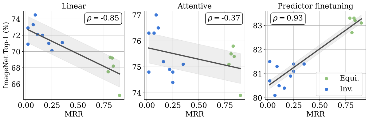
To test whether a transformation was predicted correctly, the authors rank the actual target representation among a bank of 256 transformed candidates. Mean Reciprocal Rank is high when the intended transformed target is near the top. This measures the specific transformation task; it is not classification accuracy or a physical-planning success rate.
4.2 Learning a strong Image World Model
Three choices interact. The predictor needs unambiguous transformation conditioning, an adequately challenging range of transformations and enough capacity to model their effects. Without conditioning it can instead remove transformation information. Weak transformations or an undersized predictor also encourage invariant behavior. The favored implementation mixes transformation parameters with mask-token features; its ablations compare this with sequence-token conditioning.
| Conditioning: | None | Sequence | Feature |
|---|---|---|---|
| MRR | 0.00 | 0.82 | 0.79 |
| Predictor: | I-JEPA | IWM | |
|---|---|---|---|
| (depth, dim.): | (12,384) | (12,384) | (18,384) |
| Jitter | 0.00 | 0.11 | 0.25 |
| + Destructive | 0.00 | 0.09 | 0.79 |
| + Strong Jitter | 0.00 | 0.81 | 0.85 |
4.3 Visualizing predictions.
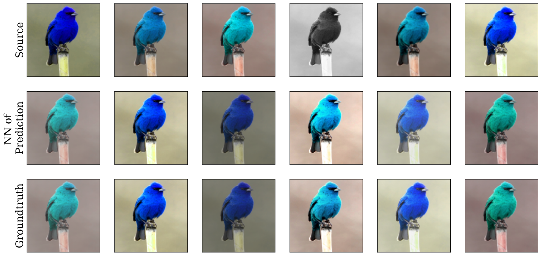
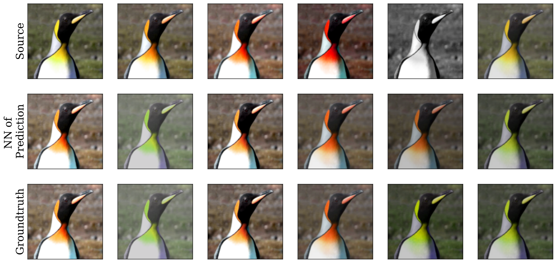
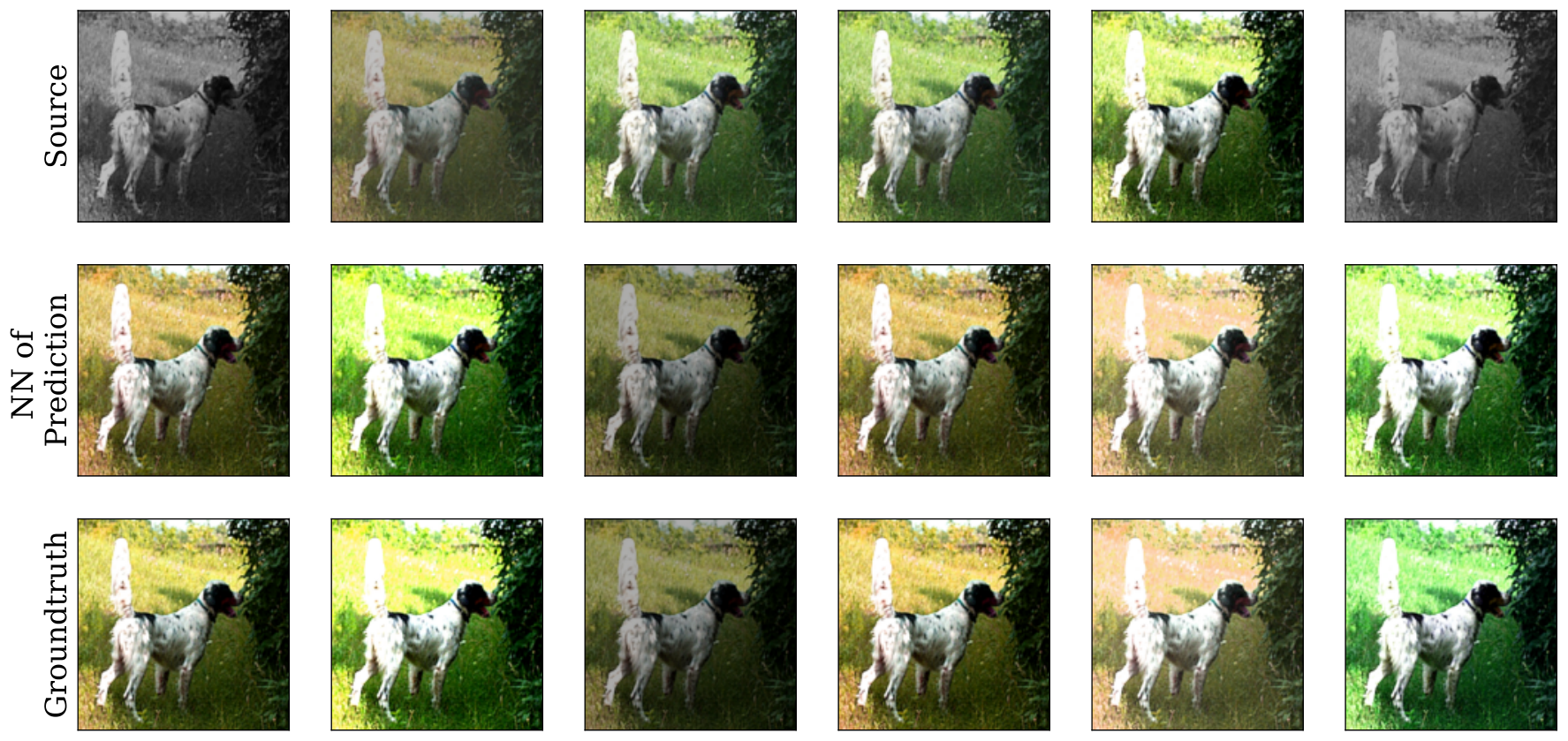
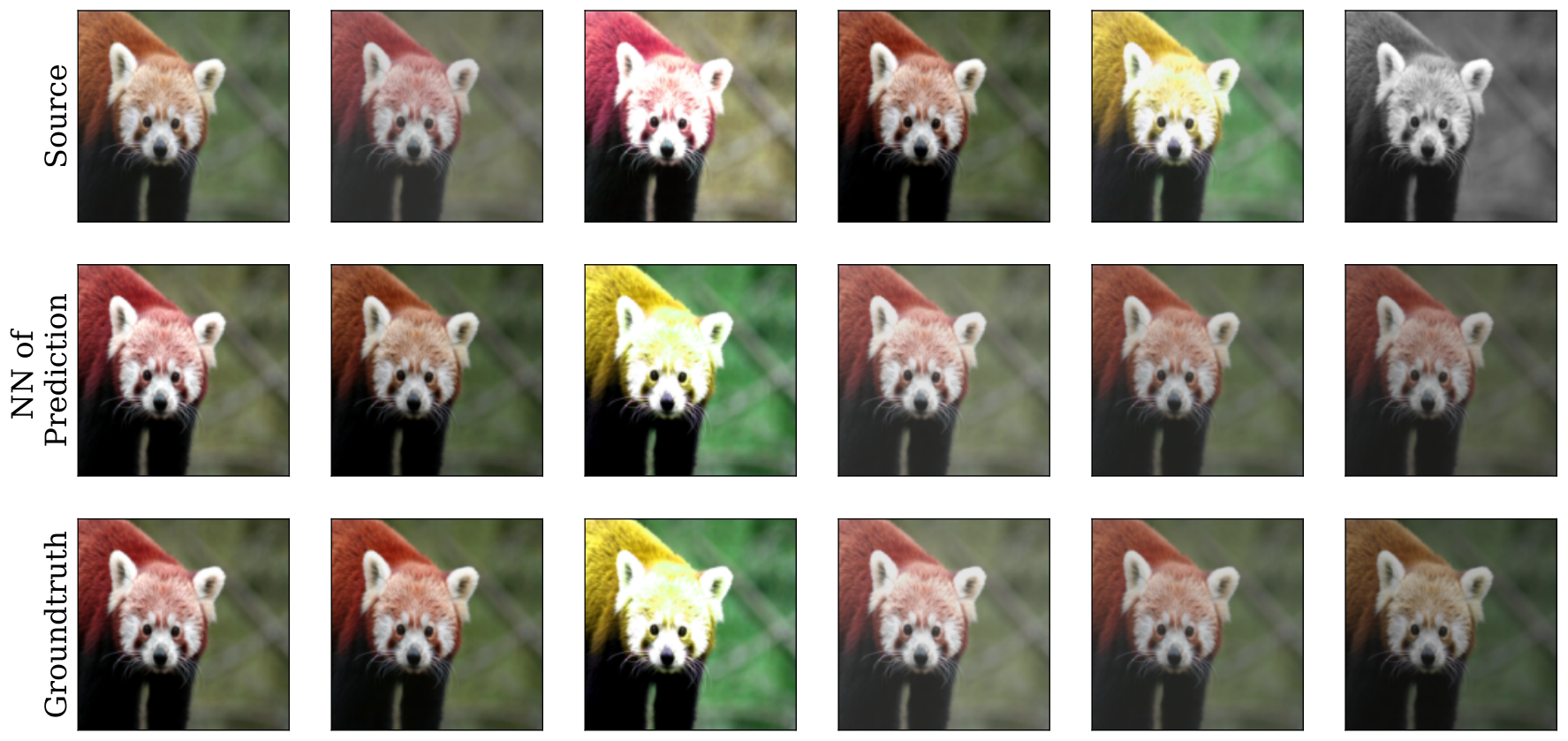
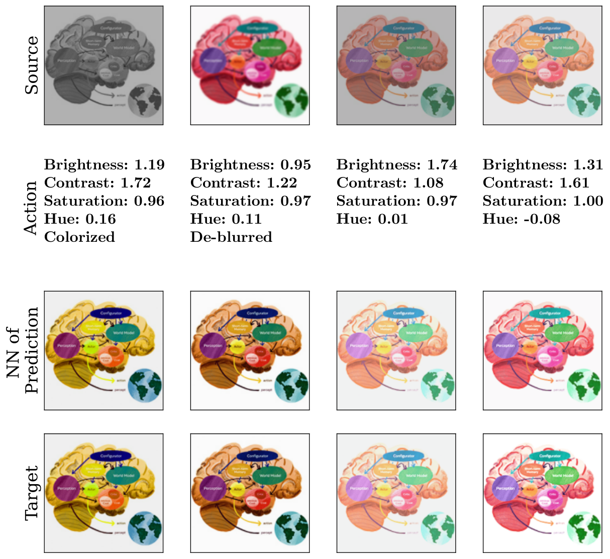
Nearest-neighbor images visualize predicted embeddings by retrieving transformed candidates. They show learned photometric changes but also ambiguity when information has been destroyed, such as recovering color from grayscale. These are representation-space retrieval visualizations, not direct pixel generation by the JEPA predictor.
5 Leveraging world models for downstream tasks
Predicting color changes is not itself the end application. The downstream experiments ask whether the world-model computation can be repurposed for image classification and semantic segmentation.
5.1 Predictor finetuning
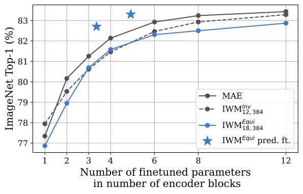
Predictor finetuning places the pretrained predictor above a frozen encoder and adapts it, with an evaluation head, to the supervised downstream task. Its pretraining output is another representation, so simply reading it without adaptation is not the same protocol. Experiments vary the target prediction task, teacher versus student features, and whether to use a pretrained or random predictor. Reusing a capable pretrained predictor can match or exceed tested encoder-finetuning baselines while avoiding encoder gradients. Comparisons must account for both predictor capacity and which parameters are trained.
| Setting | ImageNet Top-1 (%) | Gap |
|---|---|---|
| Default | 82.9 | - |
| + Teacher | 83.2 | + 0.3 |
| + Null latents | 83.3 | + 0.1 |
| + Pred only one token | 82.8 | -0.5 |
| Method | Epochs | No predictor | Frozen encoder, tuned predictor | End to end | |
|---|---|---|---|---|---|
| Encoder | Random Init. | Pretrained | |||
| MAE | 300 | 82.7 | 82.4 | 82.7 (+0.3) | 82.3 |
| 1600 | 83.6 | 83.0 | 83.1 (+0.1) | 83.3 | |
| I-JEPA | 300 | 83.0 | 79.1 | 80.0 (+0.9) | 82.0 |
| 300 | 83.3 | 80.5 | 81.3 (+0.8) | 82.7 | |
| 300 | 82.9 | 81.5 | 83.3 (+1.8) | 84.4 | |
| Method | Encoder | Predictor | End to end |
|---|---|---|---|
| I-JEPA | 44.2 | 45.4 | 45.1 |
| 45.6 | 45.7 | 46.5 | |
| 44.2 | 46.8 | 47.0 |
5.2 Multitask predictor tuning
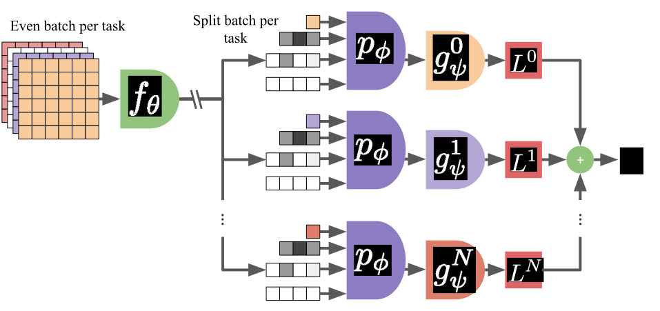
Task-specific tokens and output heads allow one predictor to be finetuned for several datasets at once. The minibatch is divided between tasks and their losses update the shared predictor. The experiment tests a particular sampling and training budget; it does not establish that adding arbitrary tasks is free or always beneficial.
| Dataset | Single-task | Multi-task | Difference |
|---|---|---|---|
| ImageNet | 80.8 | 79.6 | -1.2 |
| iNat18 | 72.4 | 72.0 | -0.4 |
| SUN397 | 75.6 | 78.2 | +2.6 |
| Places205 | 64.8 | 64.1 | -0.7 |
| Average | 73.4 | 73.5 | +0.1 |
6 Image World Models enable flexible representations
Invariant representations tend to be easier to read with a linear probe. Transformation-sensitive representations can retain richer information that an attentive head or finetuned model uses better. The paper therefore treats evaluation protocol and representation abstraction as linked choices: one linear-probe score does not determine which representation is best for every downstream use.
| Method | Effective Epochs | Linear | Attentive |
|---|---|---|---|
| MoCoV3 | 300 | 76.3 | 76.4 |
| MAE | 300 | 60.2 | 73.5 |
| MAE | 1600 | 68.0 | 76.0 |
| I-JEPA | 300 | 70.0 | 75.0 |
| 300 | 74.5 | 77.0 | |
| 300 | 67.5 | 75.1 |
7 Conclusion and future perspectives
The main design lesson is to specify which variations a representation should retain and give the predictor the information and capacity needed to model them. The demonstrated world is one of image transformations. Extending this argument to video, control or uncertain physical events requires new training data and tests.
8 Broader impact statement
The broader-impact statement presents general visual representation research and identifies no paper-specific societal consequence. This is a disclosure statement, not a deployment safety evaluation.
Appendix A Experimental details
A.1 Pretraining
Most models pretrain on ImageNet for 300 epochs with a ViT-B/16 encoder. The appendix fixes optimization, masking and augmentation schedules. Targets keep more visual information, while source views may receive destructive grayscale, blur or solarization. Momentum-target and schedule settings are part of the recipe.

A.2 Evaluation
Classification validation uses resize and center-crop preprocessing. Hyperparameters are separately tuned for the methods and evaluation protocols, so reported differences are not all from a single common optimizer setting.
Linear.
Linear evaluation average-pools frozen encoder features and trains one linear classification layer. This is the simplest readout and favors features that already make the labels linearly accessible.
Attentive.
The attentive probe learns a cross-attention pooling operation over unpooled features. It has more capacity to extract useful information than average pooling plus a linear layer, while still keeping the representation backbone frozen.
Encoder finetuning.
Encoder finetuning updates the encoder and classification head with the stated augmentation and optimizer recipe. It is a different resource and adaptation setting from training a lightweight readout.
Predictor finetuning.
Predictor finetuning uses a frozen teacher encoder, asks the predictor for the full image representation with null transformation parameters and trains an attentive task head. Pretrained predictor parameters receive a smaller learning rate than a randomly initialized predictor.
Multitask predictor finetuning.
The multitask experiment shares predictor parameters across task-specific tokens and heads. The appendix gives the balanced minibatch allocation and training budget needed to reproduce that comparison.
End to end finetuning.
End-to-end finetuning updates both encoder and predictor, with separate learning-rate scaling for pretrained components. It tests the value of further adaptation, rather than the efficiency of keeping the encoder frozen.
Segmentation.
Segmentation uses an UperNet head and ADE20K, with features from the last four encoder or predictor layers. The protocol specifies training resolution, positional interpolation at evaluation and learning-rate searches; these details affect the reported intersection-over-union scores.
Appendix B Complete finetuning results
The full table includes predictor sizes and additional baselines omitted from compact main-text comparisons. Some methods respond differently to attaching a random predictor. The proposed explanation for one weak baseline remains a hypothesis, not a verified causal finding.
| Method | Epochs | No predictor | Frozen encoder, tuned predictor | End to end | |
|---|---|---|---|---|---|
| Encoder | Random Init. | Pretrained | |||
| DINO | 1600 | 82.8 | 82.0 | N/A | 82.1 |
| MOCOv3 | 300 | 83.2 | 56.4 | N/A | 79.4 |
| iBOT | 1600 | 84.0 | 83.0 | N/A | 82.8 |
| MAE | 300 | 82.7 | 82.4 | 82.7 (+0.3) | 82.3 |
| 600 | 83.2 | 82.8 | 83.0 (+0.2) | 83.1 | |
| 1600 | 83.6 | 83.0 | 83.1 (+0.1) | 83.3 | |
| I-JEPA | 300 | 83.0 | 79.1 | 80.0 (+0.9) | 82.0 |
| 300 | 83.3 | 80.5 | 81.3 (+0.8) | 82.7 | |
| 300 | 82.7 | 81.3 | 82.7 (+1.4) | 83.3 | |
| 300 | 82.9 | 81.5 | 83.3 (+1.8) | 84.4 | |
Appendix C Impact of data augmentation
Depth and augmentation difficulty jointly affect whether a predictor learns transformation-sensitive behavior. A deeper predictor succeeds under more tested color-transformation settings; very weak augmentations can remove the pressure to learn the transformation.
| Predictor | Strengths | Probabilities | Performance | |||||||||
|---|---|---|---|---|---|---|---|---|---|---|---|---|
| Bright. | Contrast | Sat. | Hue | Jitter | Blur | Gray. | Solarize | MRR | Linear | Attentive | Pred. ft. | |
| 0.4 | 0.4 | 0.2 | 0.1 | 0.8 | 0.2 | 0.2 | 0.1 | 0.09 | 74.5 | 77.0 | 81.3 | |
| 0.4 | 0.4 | 0.2 | 0.1 | 0.8 | 0.11 | 72.1 | 76.5 | 80.5 | ||||
| 0.4 | 0.4 | 0.2 | 0.1 | 0.8 | 0.4 | 0.4 | 0.2 | 0.22 | 71.0 | 74.9 | 80.9 | |
| 0.5 | 0.5 | 0.4 | 0.2 | 0.8 | 0.2 | 0.2 | 0.1 | 0.81 | 69.3 | 75.5 | 82.7 | |
| 0.5 | 0.5 | 0.4 | 0.2 | 0.8 | 0.07 | 73.3 | 76.3 | 80.1 | ||||
| 0.2 | 0.2 | 0.1 | 0.02 | 72.9 | 76.3 | 80.7 | ||||||
| 0.4 | 0.4 | 0.2 | 0.1 | 0.8 | 0.2 | 0.2 | 0.1 | 0.79 | 67.5 | 75.1 | 83.3 | |
| 0.4 | 0.4 | 0.2 | 0.1 | 0.8 | 0.25 | 70.1 | 74.8 | 81.4 | ||||
| 0.4 | 0.4 | 0.2 | 0.1 | 0.8 | 0.4 | 0.4 | 0.2 | 0.85 | 56.1 | 74.5 | 83.1 | |
| 0.5 | 0.5 | 0.4 | 0.2 | 0.8 | 0.2 | 0.2 | 0.1 | 0.85 | 34.3 | 71.0 | 81.7 | |
| 0.5 | 0.5 | 0.4 | 0.2 | 0.8 | 0.83 | 69.2 | 75.8 | 83.3 | ||||
| 0.2 | 0.2 | 0.1 | 0.02 | 70.9 | 74.8 | 81.5 | ||||||
On the asymmetry of augmentations.
Using more destructive augmentation on the source than the target helps the tested invariant models. Transformation-sensitive models are less affected in these experiments. This suggests a robustness benefit under the tested augmentation choices, not invariance to every augmentation design.
Appendix D Impact of the prediction task on predictor finetuning performance
Additional combinations support predicting a full target representation from teacher features with flexible null conditioning during finetuning. Predicting only one token is slightly worse in the tested comparisons.
| Method | Null latents | On teacher | Pred only one token | Accuracy |
|---|---|---|---|---|
| ✓ | ✓ | 83.3 | ||
| ✓ | ✓ | ✓ | 82.8 | |
| ✓ | 83.1 | |||
| ✓ | ✓ | 82.6 | ||
| ✓ | 83.2 | |||
| ✓ | ✓ | 82.8 | ||
| 82.9 | ||||
| ✓ | 82.9 |
Appendix E Scaling to larger models
Scaling to a larger encoder also requires a sufficiently deep and wide predictor. Wider predictors introduce stability issues and sensitivity to the momentum schedule. The authors report a useful predictor-to-encoder parameter ratio for their runs; it is an empirical recipe rather than a universal scaling law.
Appendix F Evaluation on downstream datasets beyond ImageNet
Attentive probes on iNaturalist18, SUN397 and Places205 test transfer beyond ImageNet. Transformation-sensitive IWM can improve over its invariant counterpart even when it is not the best ImageNet model, reinforcing the distinction between in-domain readout simplicity and retained information useful for transfer.
| Method | ImageNet | iNat18 | SUN397 | Places205 |
|---|---|---|---|---|
| MAE | 73.5 | 50.1 | 70.2 | 60.3 |
| I-JEPA | 75.0 | 50.4 | 69.2 | 58.3 |
| 77.0 | 51.6 | 71.0 | 59.4 | |
| 75.1 | 54.2 | 71.7 | 60.5 |
Appendix G Visualizing representation differences between invariant and equivariant behavior
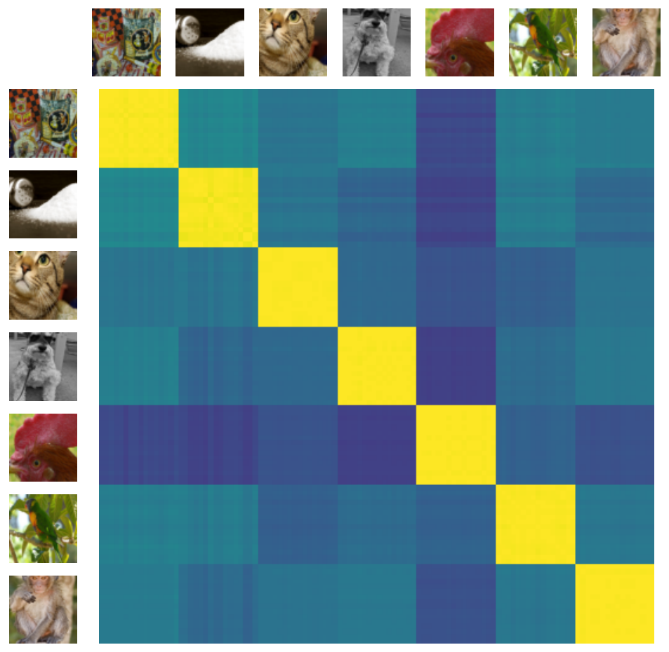
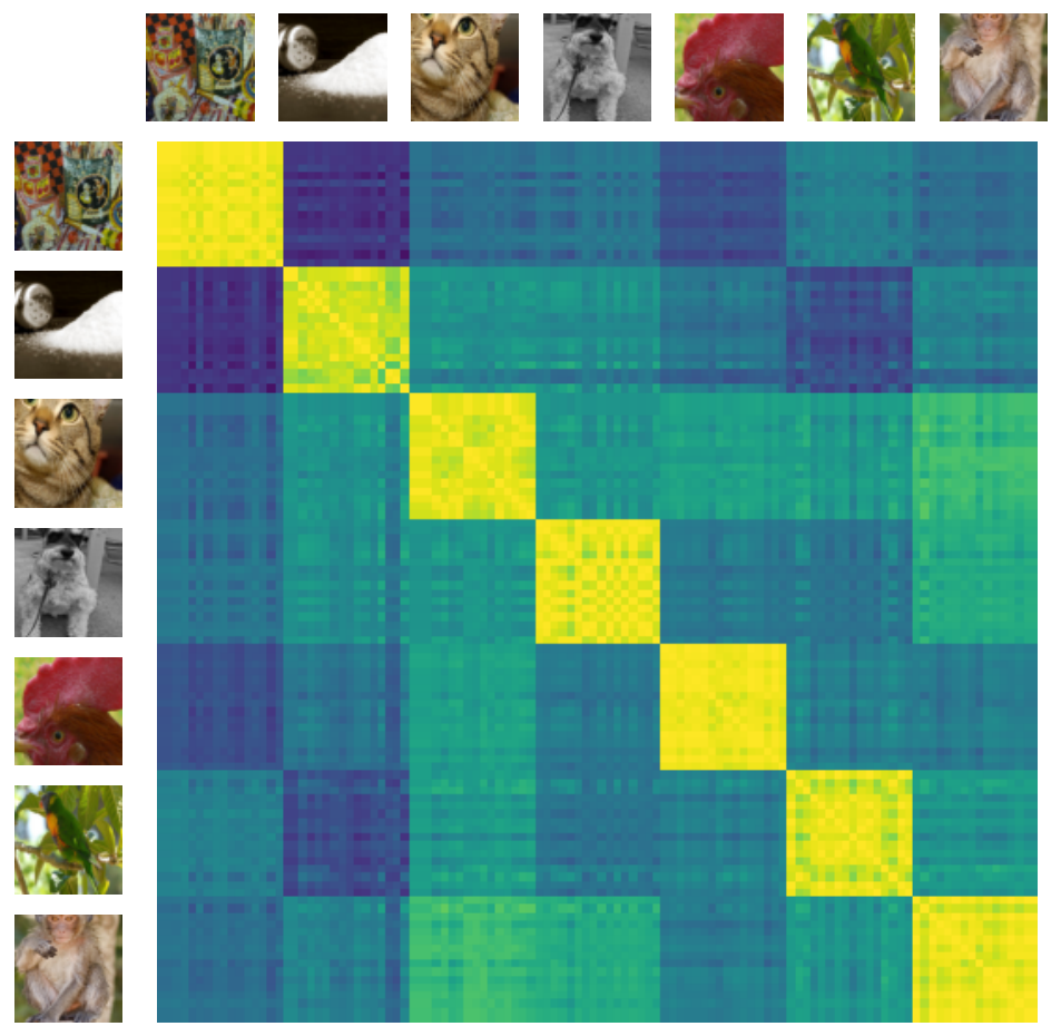
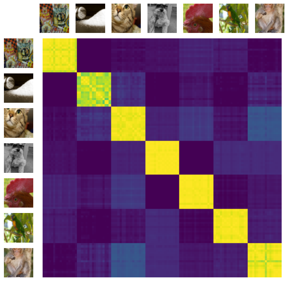
Representation-similarity visualizations show that an invariant model maps augmented views close together, while a transformation-sensitive model retains differences. I-JEPA lies between these tested behaviors rather than being explicitly optimized for either extreme.
0.3
 {subfigure}0.3
 {subfigure}0.3
Appendix H On the meaning and role of invariance in Self-Supervised learning
Invariance can arise by throwing away a changing attribute or by retaining enough information to normalize over its changes. The appendix uses IWM’s predictor to average transformed representations efficiently in latent space. Its retrieval and evaluation experiments explore this alternative while noting that invariance alone does not specify how much information was retained.
Equation
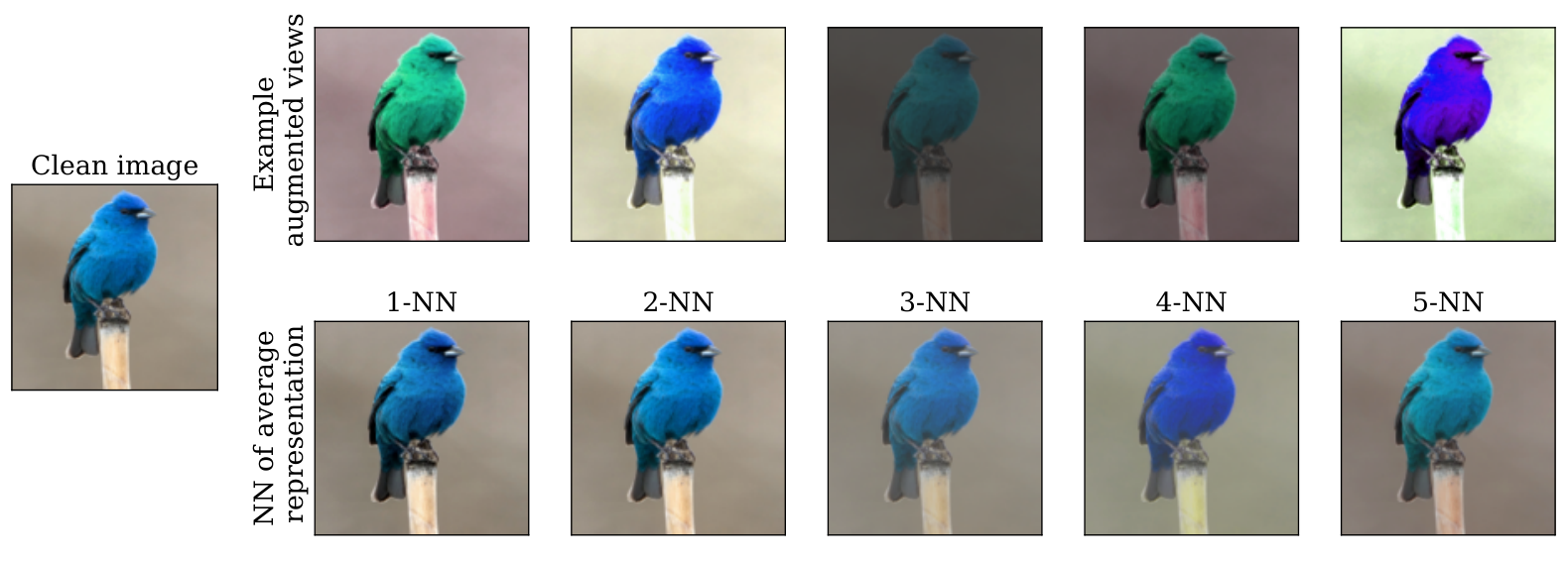
| Number of predictions () | 1 (default) | 8 | 16 | 32 | 128 |
|---|---|---|---|---|---|
| ImageNet Top-1 accuracy (%) | 64.5 | 64.3 | 64.6 | 64.6 | 64.4 |
Appendix I Additional qualitative evaluations of the world model
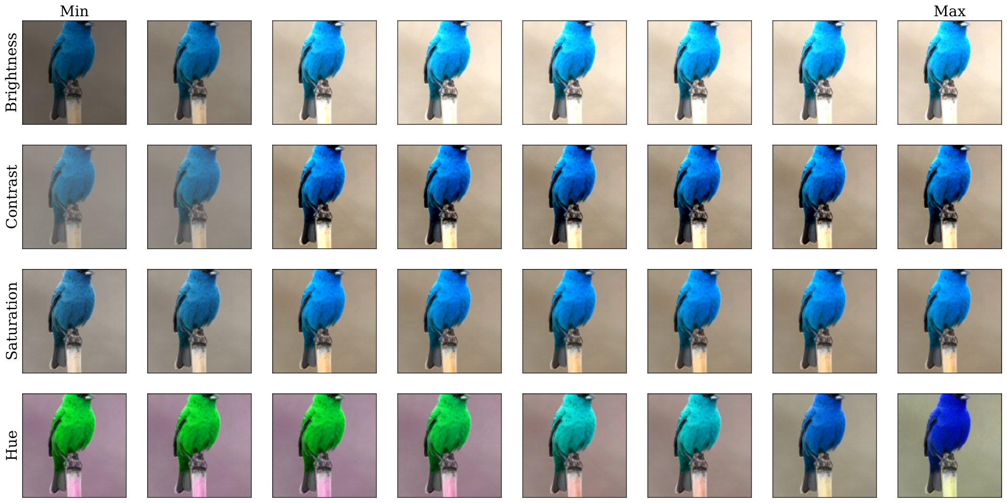
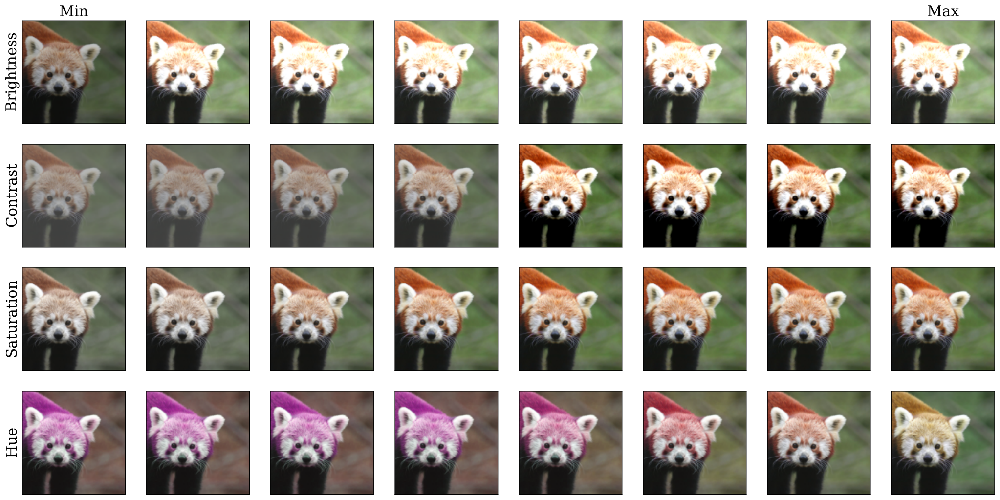
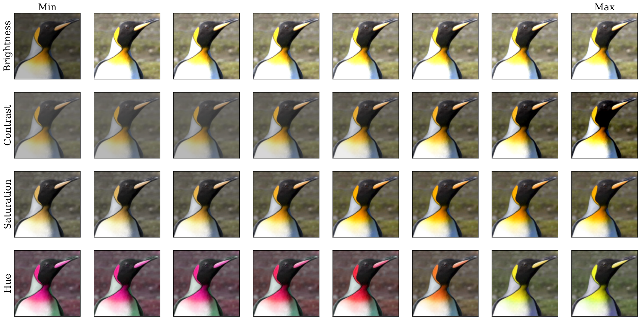
The preserved additional qualitative figures compare predicted representations with transformed image candidates. They complement the ranking metric and show both successful transformations and ambiguous destructive cases.