Literature
Display
← All papers

Neural Contractive Dynamical Systems

Hadi Beik-Mohammadi · Søren Hauberg · Georgios Arvanitidis · Nadia Figueroa · Gerhard Neumann · Leonel Rozo

· ICLR 2024 ↗

Robotics6 min text · CondensedOriginal paper ↗
Contents

At a glance

Neural Contractive Dynamical Systems (NCDS) learn motion fields by parameterizing a negative-definite matrix field and integrating it to obtain velocities. An injective variational autoencoder supports low-dimensional latent dynamics, and a restricted rotation representation extends the method to full poses. Experiments include handwriting, robot trajectories, and human motion. The paper’s stability claims concern its dynamical-system construction; decoded contraction applies on the learned manifold, with separate treatment of off-manifold initialization.

1 Stability in robot learning

Convergence to a goal does not by itself ensure that nearby motions approach one another. The authors use contraction to constrain extrapolation away from demonstrations, contrasting their architecture with mixture models, kernels, and separately learned contraction metrics. The aim is to fit flexible motion models with ordinary optimization while controlling their stability properties. [2], [31], [42].
Refer to caption
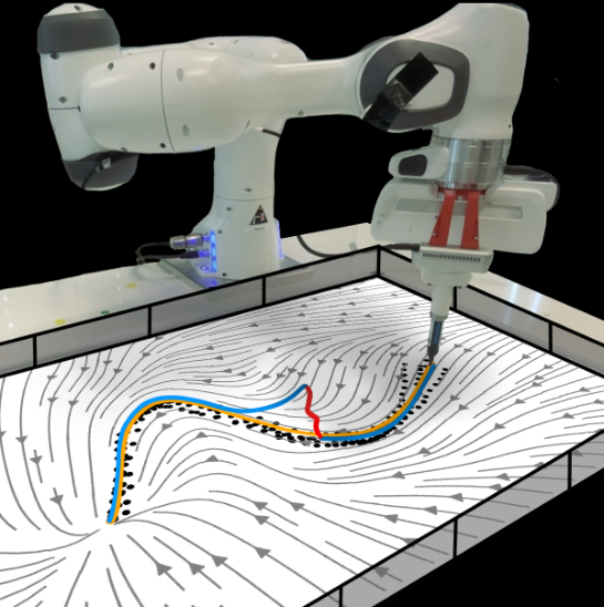
Figure 1: Robot motion executed via a neural contractive dynamical system (NCDS).

2 Learning contractive vector fields

The method begins with a differential condition for contraction and then builds a neural motion model around it.

2.1 Background: contractive dynamical systems

Uniform negativity of the symmetric part of a vector field’s Jacobian makes nearby trajectories converge exponentially in the Euclidean metric. More general contraction metrics permit state-dependent geometry; the base NCDS construction targets an identity metric.

Equations 1–2
dd​t​(δ​𝒙⊤​δ​𝒙)=2​δ​𝒙⊤​δ​𝒙˙=2​δ​𝒙⊤​𝑱​(𝒙)​δ​𝒙.\frac{\mathrm{d}}{\mathrm{d}t}(\delta\bm{x}^{\top}\delta\bm{x})=2\delta\bm{x}^{\top}\delta\dot{\bm{x}}=2\delta\bm{x}^{\top}\bm{J}(\bm{x})\delta\bm{x}. (1)
∃τ>0s.t.∀𝒙,12​(𝑱⁡(𝒙)+𝑱​(𝒙)⊤)≺−τ​𝑰≺0.\exists\,\tau>0\quad\text{s.t.}\quad\forall\bm{x},\quad\cfrac{1}{2}\Big(\bm{J}(\bm{x})+\bm{J}(\bm{x})^{\top}\Big)\prec-\tau\bm{I}\prec 0. (2)

2.2 Neural contractive dynamical systems (NCDS)

A network produces a matrix whose negative Gram matrix, shifted by a positive diagonal margin, is negative definite. The authors integrate this matrix field along a straight segment from a learned reference state to predict velocity, presenting the result as a contractive neural architecture. Training fits demonstrated velocities or next states through numerical integration.

Equation 3
𝑱f^​(𝒙)=−(𝑱𝜽​(𝒙)⊤​𝑱𝜽​(𝒙)+ϵ​𝕀D),\hat{\bm{J}_{f}}(\bm{x})=-(\bm{J}_{\bm{\theta}}(\bm{x})^{\top}\bm{J}_{\bm{\theta}}(\bm{x})+\epsilon\,\mathbb{I}_{D}), (3)
Refer to caption
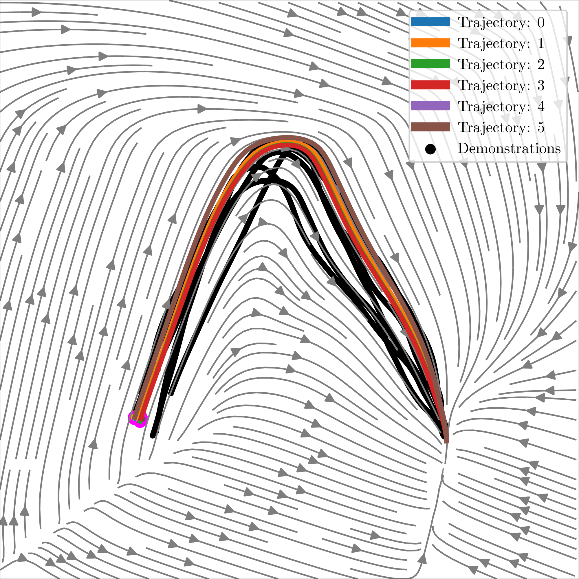
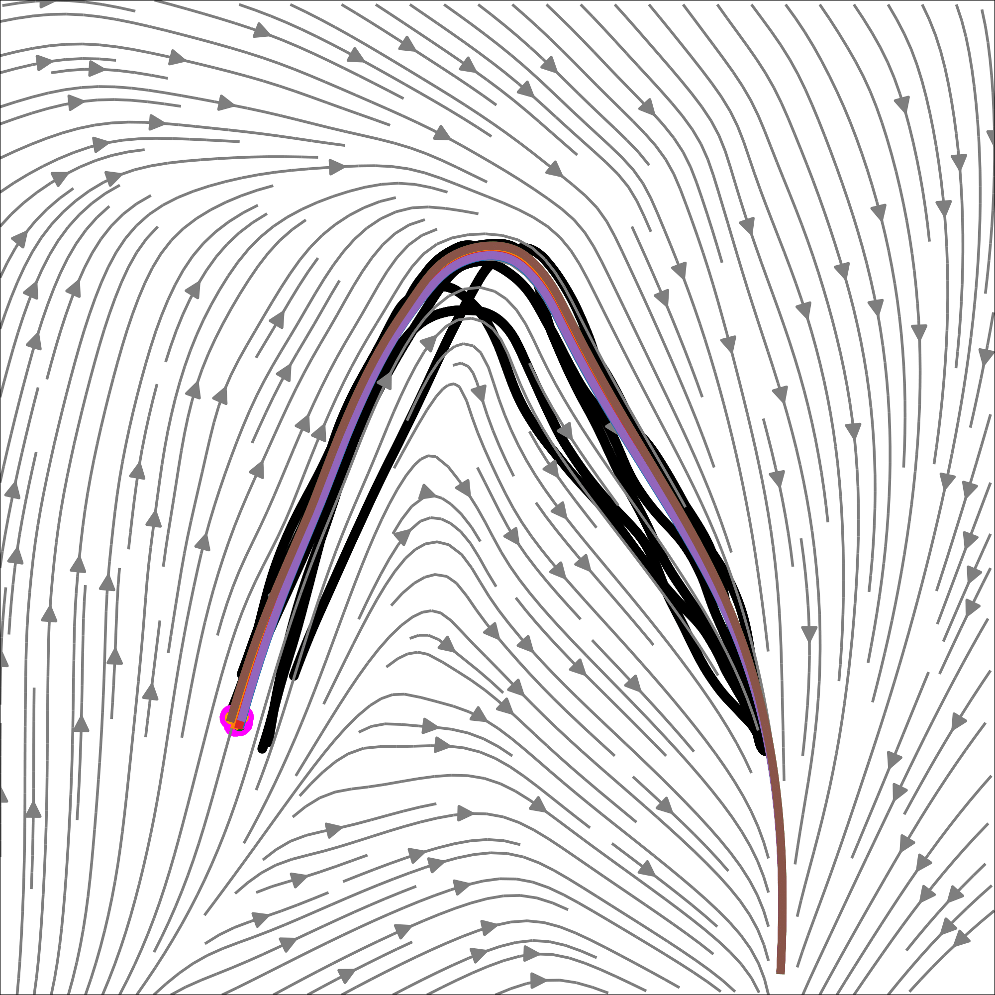
Figure 2: The learned vector field (grey) and demonstrations (black). Yellow and green trajectories show path integrals starting from demonstration starting points and random points, respectively.
Equations 4–5
𝒙˙=f⁡(𝒙)\displaystyle\dot{\bm{x}}=f(\bm{x}) =𝒙˙0+∫01𝑱f^​(c⁡(𝒙,t,𝒙0))​c˙​(𝒙,t,𝒙0)​𝑑t,\displaystyle=\dot{\bm{x}}_{0}+\int_{0}^{1}\hat{\bm{J}_{f}}\left(c\left(\bm{x},t,\bm{x}_{0}\right)\right)\dot{c}(\bm{x},t,\bm{x}_{0})\mathrm{d}t, (4)
c⁡(𝒙,t,𝒙0)\displaystyle c(\bm{x},t,\bm{x}_{0}) =(1−t)𝒙0+t𝒙andc˙(t,𝒙0,𝒙)=𝒙−𝒙0,\displaystyle=\left(1-t\right)\bm{x}_{0}+t\bm{x}\quad\text{and}\quad\dot{c}(t,\bm{x}_{0},\bm{x})=\bm{x}-\bm{x}_{0}, (5)

3 Learning latent contractive dynamics

High-dimensional models can be expensive and brittle with limited demonstrations. The latent variant learns a smaller motion space while constraining its decoder geometry.

3.1 Background: deep generative models

Variational autoencoders provide latent representations; injective flows supply the required one-to-one decoder structure.

Variational autoencoders (VAEs).

The VAE encodes observed states into a lower-dimensional distribution and learns a decoder by maximizing an evidence lower bound. Latent states serve as the inputs to the motion model.

Injective flows.

Zero-padding followed by invertible transformations embeds a low-dimensional latent space into a higher-dimensional observation space without self-intersections.

3.2 Latent neural contractive dynamical systems

The injective decoder is a diffeomorphism onto its image, allowing the paper’s contraction argument to transfer to that learned manifold. Its Jacobian maps latent velocities into observation-space velocities. Off-manifold initial states are projected through an approximate encoder; the initial movement to the manifold is explicitly not guaranteed to be contractive.

Equations 6–8
μ=gK∘⋯∘g1∘Pad,\displaystyle\mu=g_{K}\circ\cdots\circ g_{1}\circ\operatorname{Pad}, (6)
μ∼1𝝃=Unpad∘g1−1∘⋯∘gK−1,\displaystyle\mu^{\sim 1}_{\bm{\xi}}=\operatorname{Unpad}\circ\,g_{1}^{-1}\circ\cdots\circ g_{K}^{-1}, (7)
𝒙˙=𝑱μ𝝃​(𝒛)​𝒛˙.\dot{\bm{x}}=\bm{J}_{\mu_{\bm{\xi}}}(\bm{z})\dot{\bm{z}}. (8)

3.3 Learning position and orientation dynamics

Full-pose motion combines Euclidean positions with rotation geometry.

Orientation parameterization.

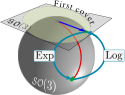
Rotation matrices lie on SO(3). Logarithmic and exponential maps relate them to three-dimensional rotation vectors, but wrapping prevents a globally one-to-one parameterization. The method restricts vectors to norms below π.
Refer to caption
Figure 3: Aspects of the Lie group 𝒮​𝒪​(3)\mathcal{SO}(3).

NCDS on Lie groups.

An injective decoder constrained to the open π-ball is followed by the rotation exponential map. Position and rotation coordinates can then share latent dynamics while retaining the stated coordinate-change argument within this restricted representation.
Refer to caption
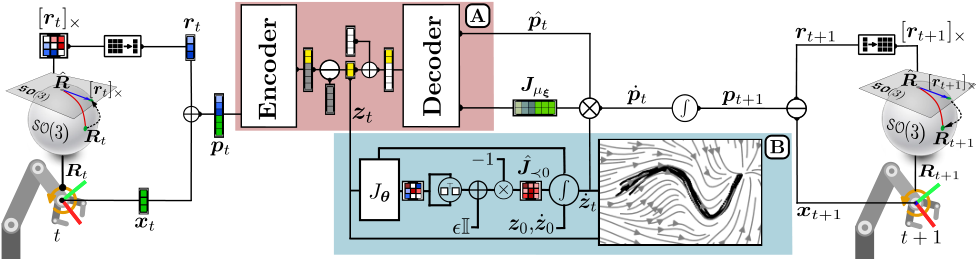
Figure 4: Architecture overview: a single iteration of NCDS simultaneously generating position and orientation dynamics. (A) VAE (pink box): The encoder processes the concatenated position-orientation data 𝒑t{\bm{p}}_{t}, yielding a resulting vector that is subsequently divided into two components: the latent code 𝒛{\bm{z}} (yellow squares) and the surplus (gray squares). The Unpad\operatorname{Unpad} function in Equation 7 removes the unused segment. The unpadded latent code 𝒛{\bm{z}} is fed to the contraction module and simultaneously padded with zeros (white squares) before being passed to the injective decoder. (B) Contraction (blue box): The Jacobian network output, given the latent codes, is reshaped into a square matrix and transformed into a negative definite matrix using Equation 2. The numerical integral solver then computes the latent velocity 𝒛˙\dot{{\bm{z}}}. Later, using Eq. 8, 𝒛˙\dot{{\bm{z}}} is mapped to the input-space velocity via the decoder’s Jacobian 𝑱​μ𝝃\bm{J}{\mu_{\bm{\xi}}}.

3.4 Obstacle avoidance via matrix modulation

Obstacle geometry and position define a modulation matrix that reshapes the decoded velocity field near obstacles. The paper invokes prior modulation theory for stability preservation. The demonstrated construction avoids obstacles at the end effector; whole-body avoidance requires additional modeling. [12].

4 Experimental results

Evaluation emphasizes reconstruction accuracy, nearby-trajectory behavior, higher-dimensional representations, and qualitative robot recovery.

Datasets.

Ten LASA handwriting shapes are selected and preprocessed to share endpoint conventions. Stacking shapes creates four- and eight-dimensional datasets. Further data include five seven-joint robot trajectories and kinesthetic end-effector demonstrations.

Metrics.

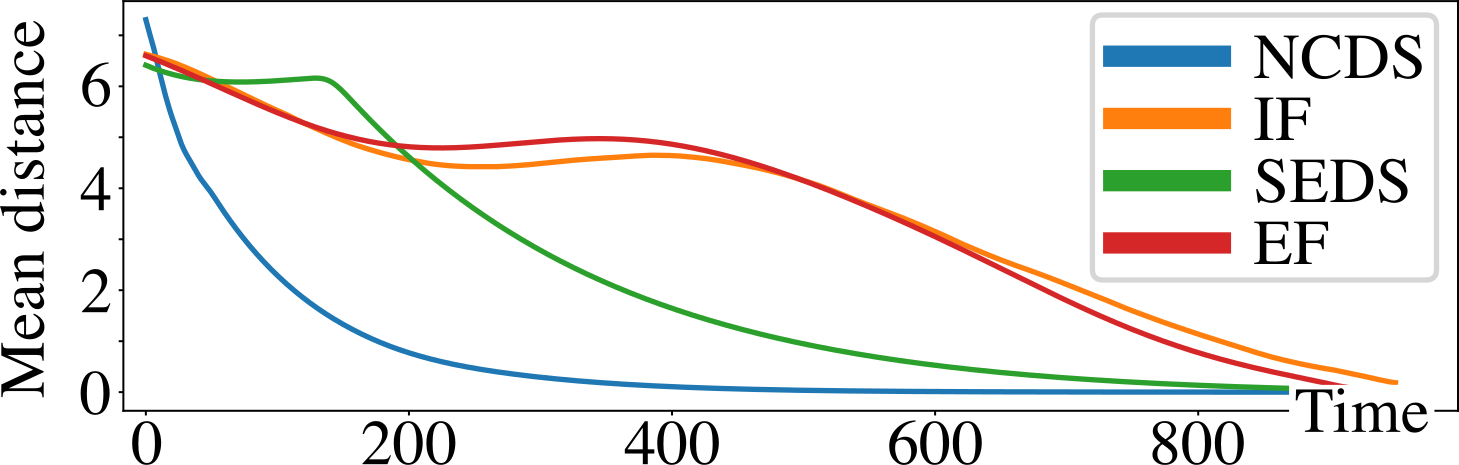
Reconstruction is measured using the paper’s stated DTWD formula, which sums nearest-point distances in both trajectory directions. Nearby-trajectory distance over time is also plotted to assess contraction behavior.

Equation
DTWD⁡(τx,τx′)=∑j∈l⁡(τx′)mini∈l⁡(τx)⁡(d⁡(τxi,τxj′))+∑i∈l⁡(τx)minj∈l⁡(τx′)⁡(d⁡(τxi,τxj′)),\operatorname{DTWD}({\tau_{x}},\tau_{{x}^{\prime}})=\sum_{j\in l({\tau}_{x^{\prime}})}\min_{i\in l(\tau_{x})}\left(d(\tau_{x_{i}},{\tau}_{x_{j}^{\prime}})\right)+\sum_{i\in l(\tau_{x})}\min_{j\in l({\tau}_{x^{\prime}})}\left(d(\tau_{x_{i}},{\tau}_{x_{j}^{\prime}})\right),

Baseline methods.

Euclideanizing Flow, Imitation Flow, and SEDS are comparison methods with asymptotic stability objectives; they do not target the same contraction guarantee.

4.1 Comparative results

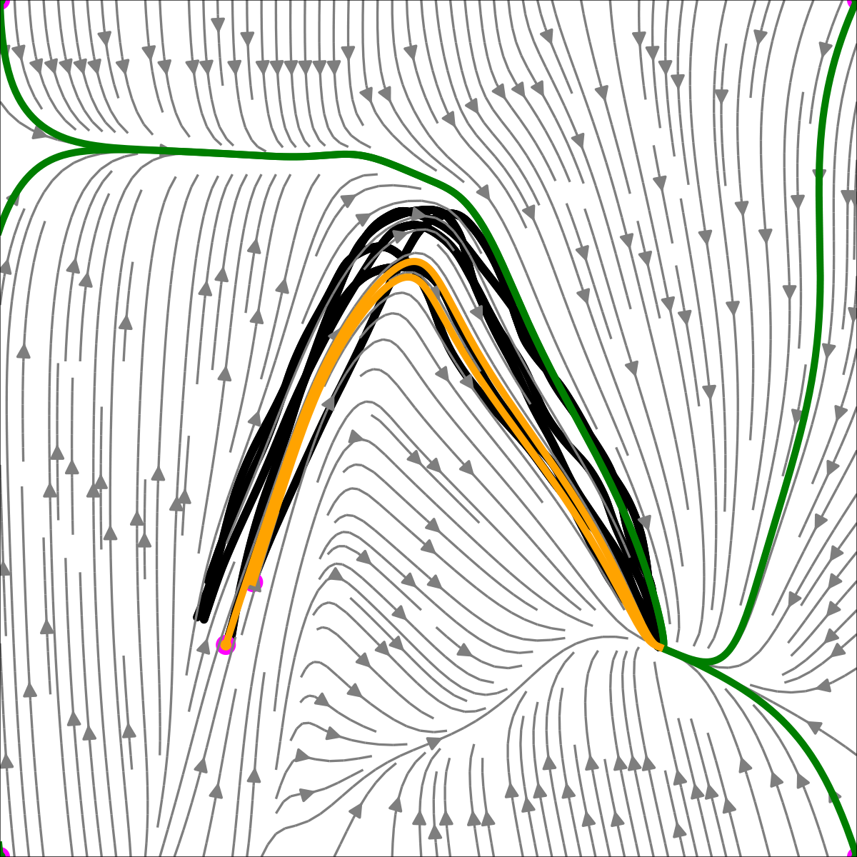
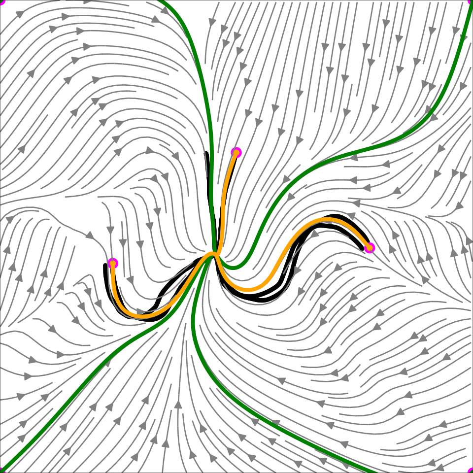
NCDS is not most accurate in low dimensions: Euclideanizing Flow wins on LASA-2D and Imitation Flow on LASA-4D. NCDS has the lowest reported DTWD on LASA-8D (2.28 ± 0.24) and seven-joint data (1.18 ± 0.16). The latent representation is central to these higher-dimensional gains.
Refer to caption
Original figure
Refer to caption
Refer to caption
Refer to caption
Refer to caption
Refer to caption
Refer to caption
Refer to caption
Refer to caption
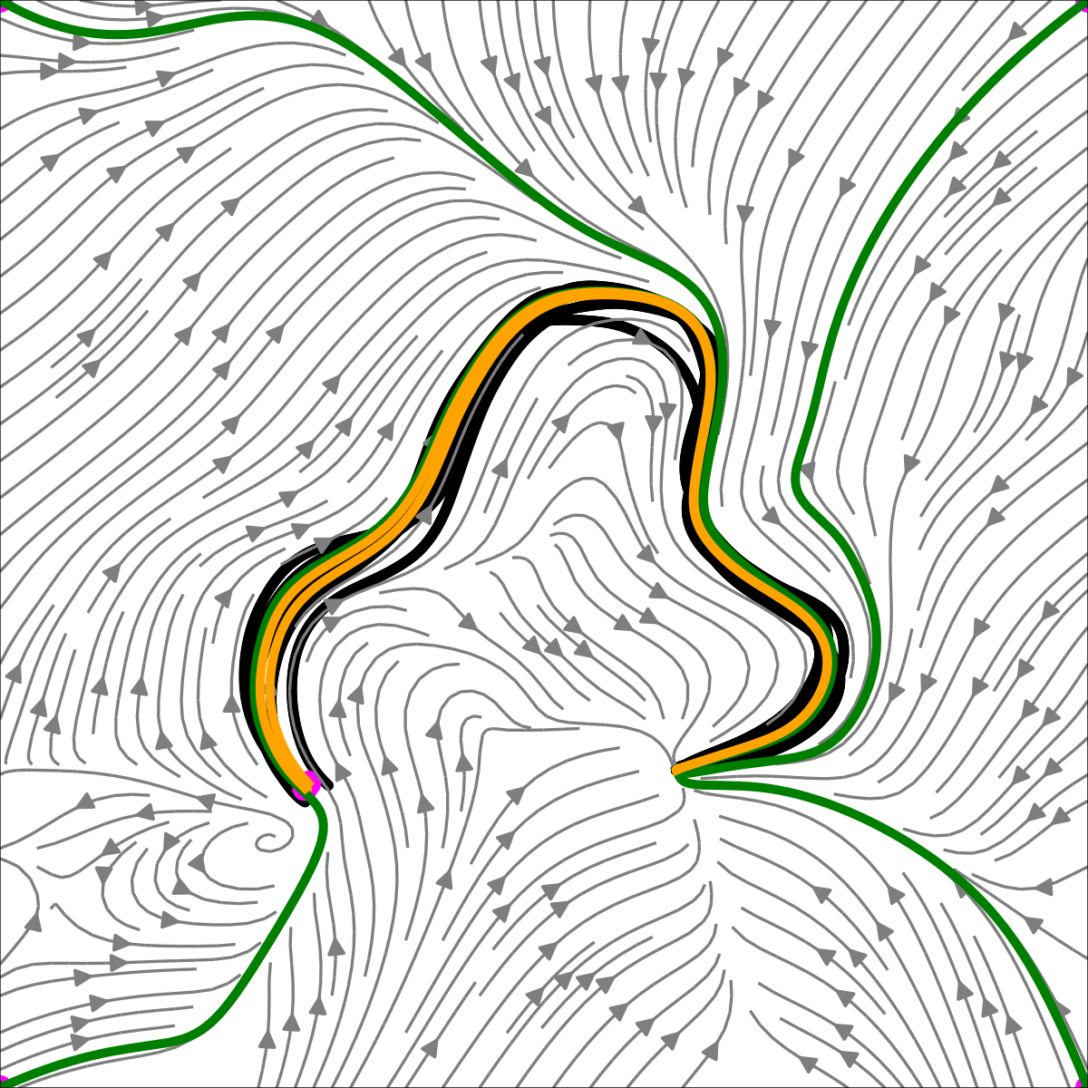
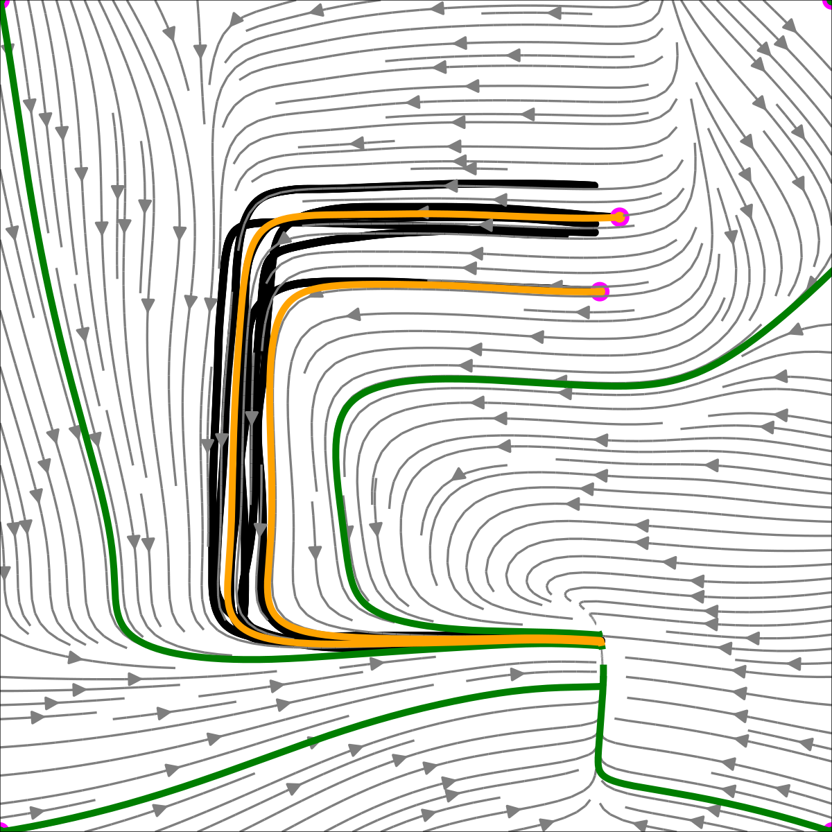
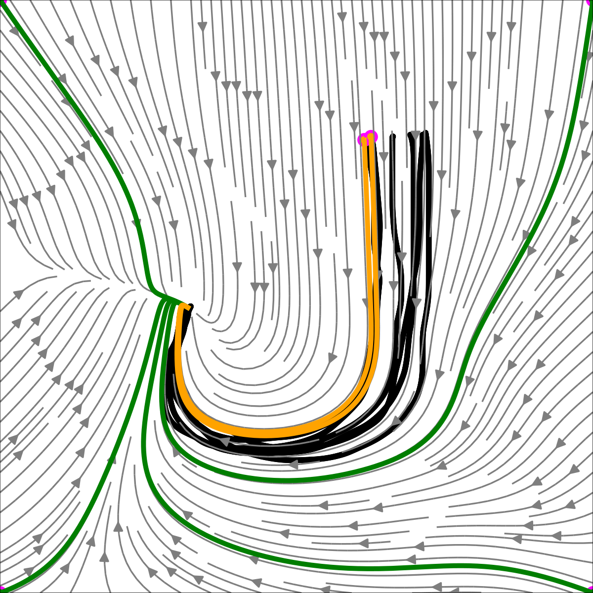
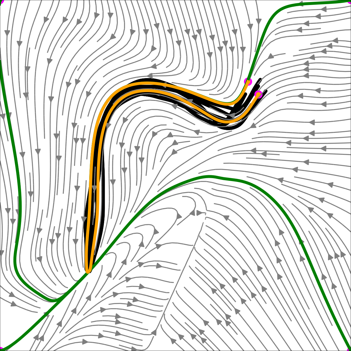
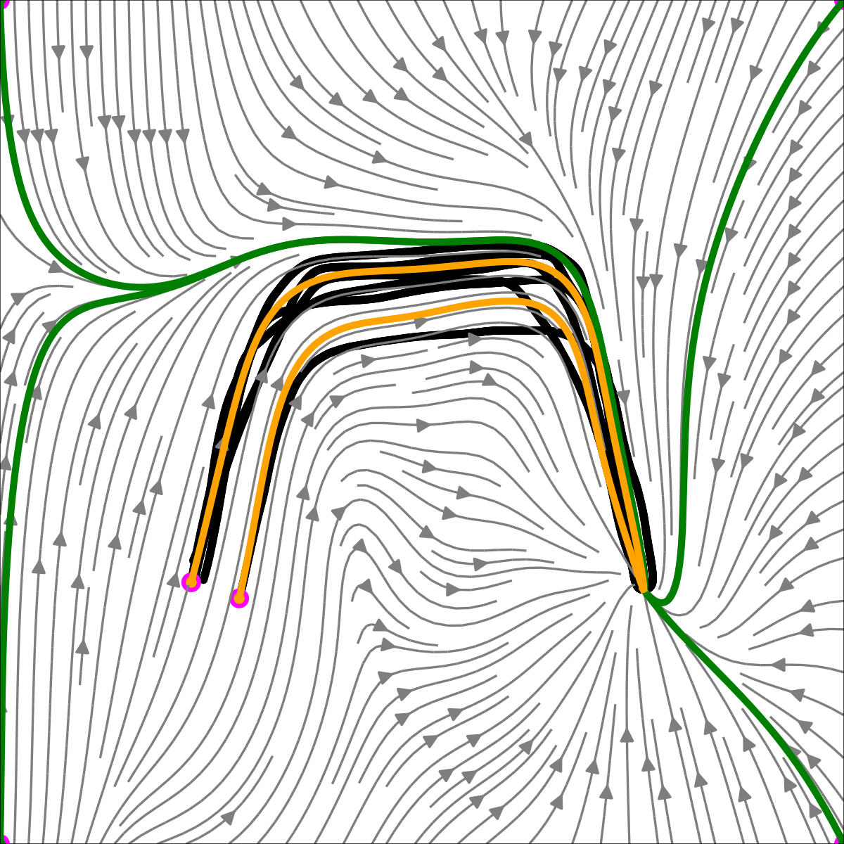
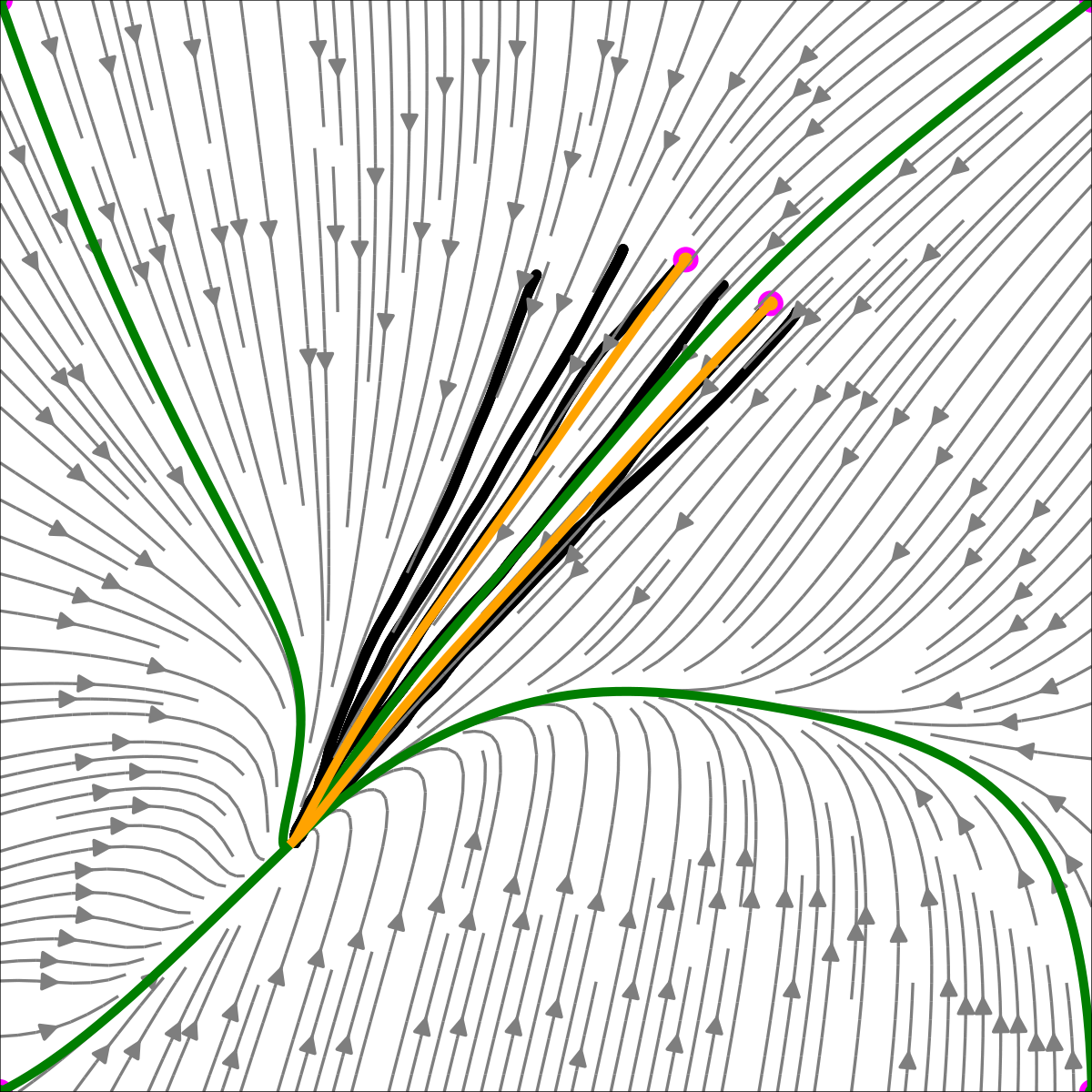
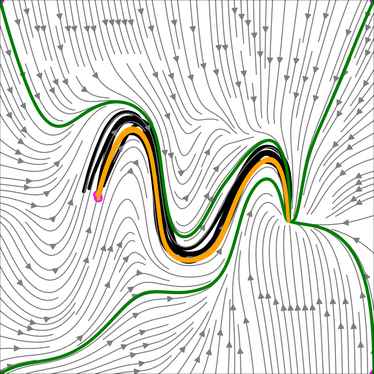
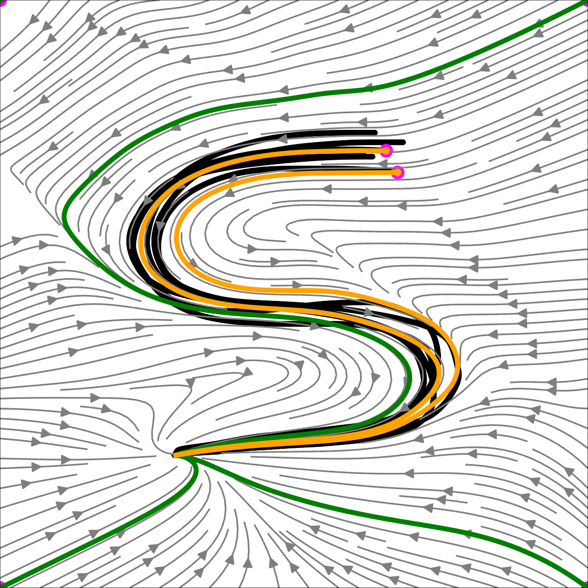
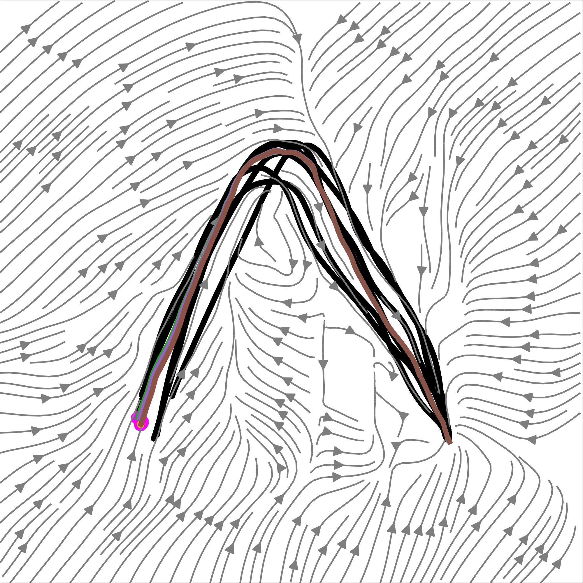
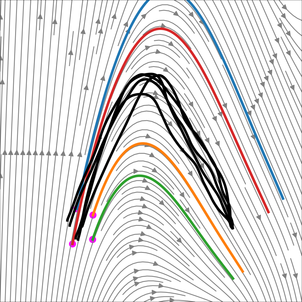
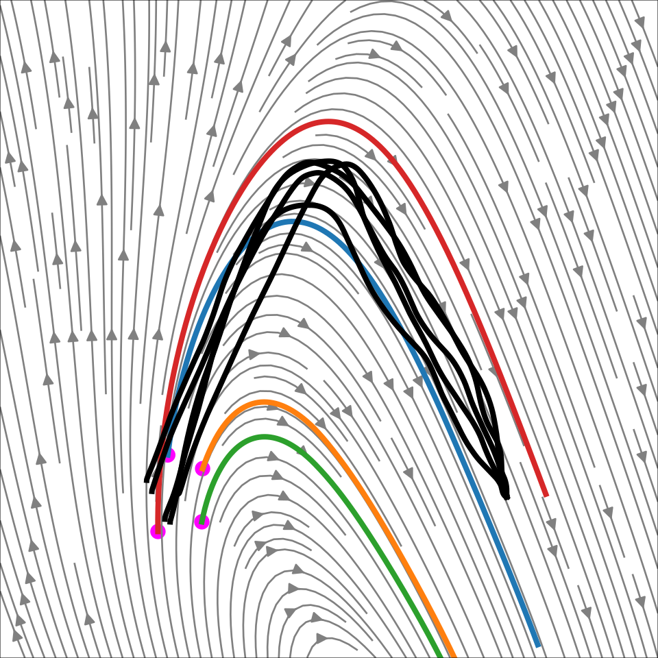
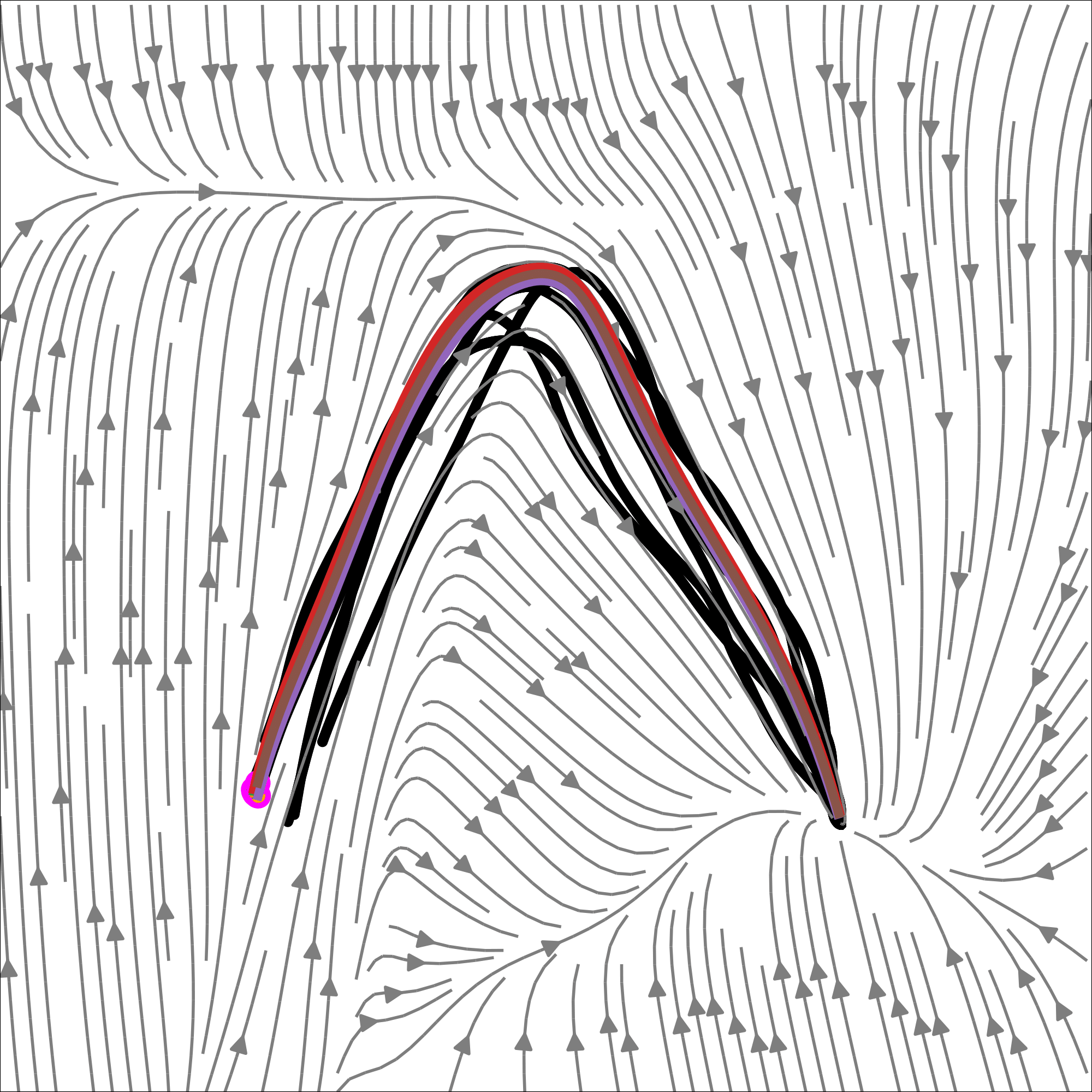
Figure 5: Visualization of the LASA-2D dataset: Gray contours represent the learned vector field, black trajectories depict demonstrations, and orange/green trajectories illustrate path integrals starting from the initial points of the demonstrations and plot corners. The magenta circles indicate the initial points of the path integrals.
Original figure
Figure 6: Average distance between random nearby trajectories over time for LASA-2D. Only NCDS monotonically decreases, i.e. it is the only contractive method.
Original figure
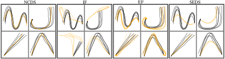
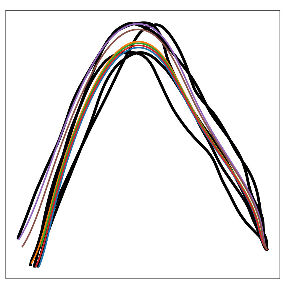
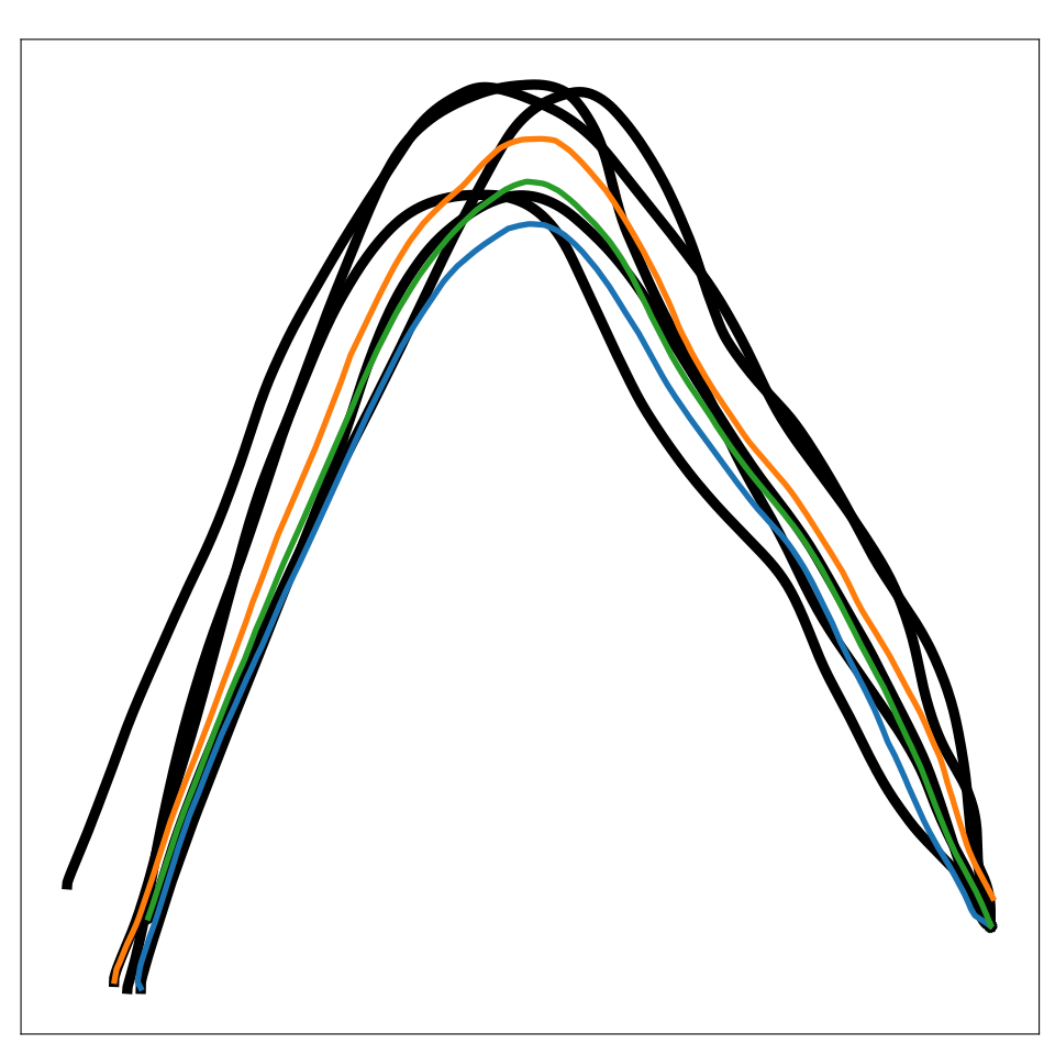
Figure 7: Path integrals generated using different methods on LASA-8D. Black curves are training data, while yellow are the learned path integrals. To construct the 8D dataset, we have concatenated 4 different 2D datasets.
LASA-2D LASA-4D LASA-8D 7 DoF robot
Euclideanizing flow 0.72±0.12\textbf{0.72}\pm\textbf{0.12} 3.23±0.343.23\pm 0.34 10.22±0.4010.22\pm 0.40 5.11±0.305.11\pm 0.30
Imitation flow 0.80±0.240.80\pm 0.24 0.79±0.22\textbf{0.79}\pm\textbf{0.22} 4.69±0.524.69\pm 0.52 2.63±0.372.63\pm 0.37
SEDS 1.60±0.441.60\pm 0.44 3.08±0.203.08\pm 0.20 4.85±1.644.85\pm 1.64 2.69±0.182.69\pm 0.18
NCDS 1.37±0.401.37\pm 0.40 0.98±0.150.98\pm 0.15 2.28±0.24\textbf{2.28}\pm\textbf{0.24} 1.18±0.16\textbf{1.18}\pm\textbf{0.16}
Table 1: Average dynamic time warping distances (DTWD) between different approaches. NCDS exhibits comparable performance in low dimensions, while clearly being superior in high dimensions.

4.2 Obstacle avoidance

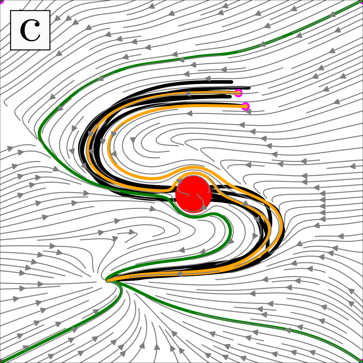
Handwriting fields and a robot demonstration show trajectories rerouting around a known obstacle while reaching the target. These are controlled demonstrations of the modulation method, not a broad collision-safety benchmark.

4.3 Robot experiment

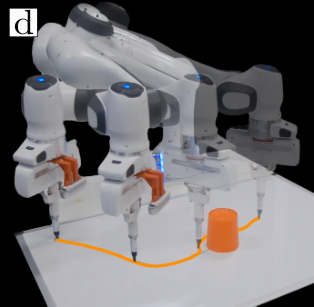
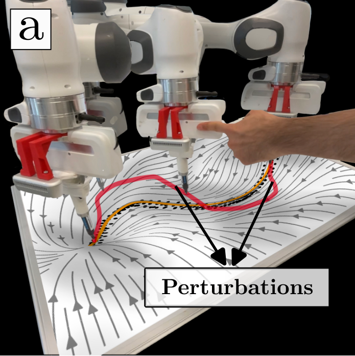
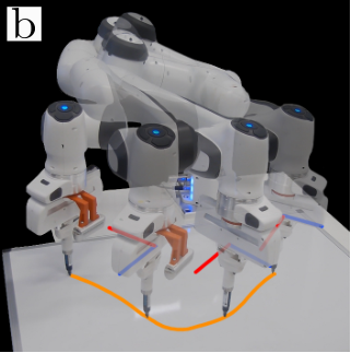
A Franka arm reproduces taught sinusoidal and V-shaped motions using Cartesian impedance control, including manually perturbed executions. Additional experiments cover synthetic position-orientation data, simulated joint-space reproduction, and human-motion trajectories.
Refer to caption
Refer to caption
Refer to caption
Refer to caption
Figure 8: Robot and obstacle avoidance. Left two panels show robot experiments with orange and red paths illustrating unperturbed and perturbed motion. The first panel shows a learned vector field in ℝ3\mathbb{R}^{3} with a constant orientation. In the second panel, the vector field expands to ℝ3×𝒮​𝒪​(3)\mathbb{R}^{3}\times\mathcal{SO}(3), aligning the end-effector’s orientation with the motion direction. Superimposed robot images depict frames of executed motion. s The right two panels display how an obstacle locally reshapes the learned vector field using the modulation matrix. In the third panel, gray contours represent the learned vector field, black trajectories depict the demonstrations, and orange/green trajectories are path integrals starting from both initial points of the demonstrations and plot corners. Magenta and red circles indicate the initial points of the path integrals and the obstacle, correspondingly. The last panel shows how the robot successfully avoids the obstacle (orange cylinder).

5 Discussion

The architecture combines a constrained matrix-field model, latent representation, orientation handling, and optional obstacle modulation. The evidence supports useful motion reproduction in the tested settings, with numerical and representation assumptions limiting the scope of its guarantees.

Limitations.

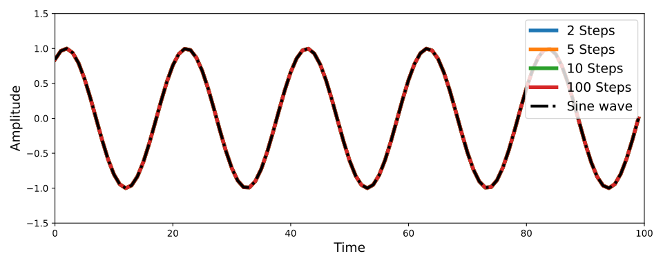
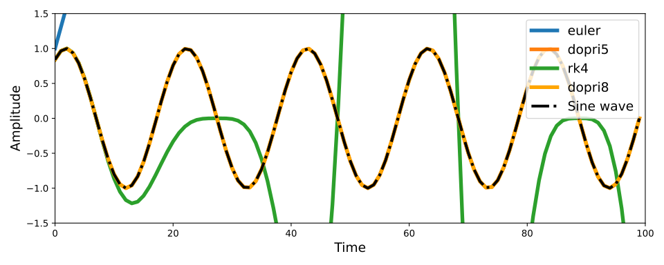
Results are sensitive to the integration scheme. Adaptive stepping improves reliability but adds computation and variable latency; high-dimensional queries may not meet strict real-time requirements.

Acknowledgments

The work acknowledges VILLUM FONDEN, the European Research Council, and the Novo Nordisk Foundation.

Appendix A Appendix

The appendix retains mathematical details, algorithms, architectural choices, and additional comparisons.

A.1 Negative Definiteness of a Symmetric Matrix

The appendix relates a symmetric matrix’s negative-definite quadratic form to its eigenvalues, supporting the matrix parameterization used in the method.

A.2 Lie operators of 𝒮 ​ 𝒪 ​ ( 3 )

Closed-form logarithmic and exponential maps specify the rotation representation and its angle-dependent terms.

Equations 9–10
Exp⁡([𝒓]×)\displaystyle\operatorname{Exp}([\bm{r}]_{\times}) =𝕀+sin⁡(ζ)ζ​[𝒓]×+1−cos⁡(ζ)ζ2​[𝒓]×2,\displaystyle=\mathbb{I}+\frac{\sin(\zeta)}{\zeta}[\bm{r}]_{\times}+\frac{1-\cos(\zeta)}{\zeta^{2}}[\bm{r}]_{\times}^{2}, (9)
Log⁡(𝑹)\displaystyle\operatorname{Log}(\bm{R}) =ζ​𝑹−𝑹⊤2​sin⁡(ζ),\displaystyle=\zeta\frac{\bm{R}-\bm{R}^{\top}}{2\sin(\zeta)}, (10)

A.3 Obstacle avoidance via matrix modulation

The modulation matrix changes radial and tangential velocities according to a differentiable obstacle-distance function and reactivity parameter. Known obstacle geometry is required, and the authors cite the prior method’s stability analysis.

Equations 11–12
𝒙˙=𝑮⁡(𝒙)​𝑱μ𝝃​(𝒛)​𝒛˙,with𝑮⁡(𝒙)=𝑬⁡(𝒙)​𝑫​(𝒙)​𝑬​(𝒙)−1,\dot{\bm{x}}=\bm{G}(\bm{x})\bm{J}_{\mu_{\bm{\xi}}}(\bm{z})\dot{\bm{z}},\quad\text{with}\quad\bm{G}(\bm{x})=\bm{E}(\bm{x})\bm{D}(\bm{x})\bm{E}(\bm{x})^{-1}, (11)
𝑬⁡(𝒙)=[r⁡(𝒙)​𝐞1​(𝒙)​…​𝐞d−1​(𝒙)],and𝑫⁡(𝒙)=diag​(λr​(𝒙)​λe​(𝒙),…,λe​(𝒙)),\bm{E}(\bm{x})=[r(\bm{x})\ \mathbf{e}_{1}(\bm{x})\ldots\mathbf{e}_{d-1}(\bm{x})],\quad\text{and}\quad\bm{D}(\bm{x})=\text{{diag}}(\lambda^{r}(\bm{x})\lambda^{e}(\bm{x}),\ldots,\lambda^{e}(\bm{x})), (12)

A.4 Implementation Details

The injective decoder uses three rational-quadratic spline coupling layers with small residual networks. The Jacobian network has two 500-unit hidden layers. PyTorch and torchdiffeq implement training and numerical integration.

Loss functions:

The VAE uses the evidence lower bound, including a Kullback–Leibler term. The motion model then minimizes latent next-state reconstruction error.

Equations 13–14
ℒE​L​B​O=𝔼q𝝃​(𝒛|𝒙)[log(pϕ(𝒙|𝒛))]−KL(q𝝃(𝒛|𝒙)||p(𝒛)),\mathcal{L}_{ELBO}=\mathbb{E}_{q_{\bm{\xi}}(\bm{z}|\bm{x})}\left[\log(p_{\bm{\phi}}(\bm{x}|\bm{z}))\right]-\mathrm{KL}\left(q_{\bm{\xi}}(\bm{z}|\bm{x})||p(\bm{z})\right), (13)
ℒJac=‖𝒛t+1−(𝒛t+𝒛˙^t)‖2,\mathcal{L}_{\text{Jac}}=\|\bm{z}_{t+1}-(\bm{z}_{t}+\hat{\dot{\bm{z}}}_{t})\|^{2}, (14)

Algorithms:

Training occurs in stages: fit the VAE, encode demonstrations, estimate latent velocities, and fit the NCDS model. At execution, encode the pose, predict latent velocity, and apply the decoder Jacobian. Both original algorithms are retained.
Algorithm 1 Neural Contractive Dynamical Systems (NCDS): Training in task space
Data: Demonstrations: τn={(𝒙t,𝑹t)}n,n∈[1,N],t∈[1,Tn]\tau_{n}=\left\{(\bm{x}_{t},\bm{R}_{t})\right\}_{n},n\in[1,N],t\in[1,T_{n}]
Result: Learned contractive dynamical system
𝒓n,t=Log⁡(𝑹n,t)\bm{r}_{n,t}=\operatorname{Log}(\bm{R}_{n,t}); // Obtaining skew-symmetric coefficients via the Lie algebra
𝒑n,t=[𝒙n,t,𝒓n,t]\bm{p}_{n,t}=[\bm{x}_{n,t},\bm{r}_{n,t}]; // Create new state vector
argmin𝝃​ℒELBO​(𝝃∗,𝒑n,t)\text{argmin}_{\bm{\xi}}\mathcal{L}_{\text{ELBO}}(\bm{\xi}^{*};\bm{p}_{n,t}); // Train the VAE
𝒛n,t=μ𝝃∼1​(𝒑n,t)\bm{z}_{n,t}=\mu_{\bm{\xi}}^{\sim 1}(\bm{p}_{n,t}); // Encode all poses using the trained VAE
𝒛˙n,t=𝒛n,t+1−𝒛n,tΔ​t\dot{\bm{z}}_{n,t}=\frac{\bm{z}_{n,t+1}-\bm{z}_{n,t}}{\Delta t}; // Estimate latent velocities via finite differences
argmin𝜽​ℒJac​(𝜽∗,𝒑n,t)\text{argmin}_{\bm{\theta}}\mathcal{L}_{\text{Jac}}(\bm{\theta}^{*};\bm{p}_{n,t}); // Train the Jacobian network
Algorithm 2 Neural Contractive Dynamical Systems (NCDS): Robot Control Scheme
Data: Current state of the robot end-effector at time tt: [𝒙t,𝑹t][\bm{x}_{t},\bm{R}_{t}]
Result: Velocity of the end-effector at current time step 𝒙˙t\dot{\bm{x}}_{t}
𝒓t=Log⁡(𝑹t)\bm{r}_{t}=\operatorname{Log}(\bm{R}_{t}); // Obtaining skew-symmetric coefficients
𝒑t=[𝒙t,𝒓t]\bm{p}_{t}=[\bm{x}_{t},\bm{r}_{t}]; // Create new state vector
𝒛t=μ𝝃∼1​(𝒑t)\bm{z}_{t}=\mu_{\bm{\xi}}^{\sim 1}(\bm{p}_{t}); // Compute the latent state
𝒛˙^t=f⁡(𝒛t)\hat{\dot{\bm{z}}}_{t}=f(\bm{z}_{t}); // Compute the latent velocity
𝑱μ𝝃​(𝒛t)=∂μ𝝃∂𝒛t\bm{J}_{\mu_{\bm{\xi}}}(\bm{z}_{t})=\frac{\partial\mu_{\bm{\xi}}}{\partial\bm{z}_{t}}; // Compute the Jacobian of the decoder
𝒙˙t=𝑱μ𝝃​(𝒛t)​𝒛˙^t\dot{\bm{x}}_{t}=\bm{J}_{\mu_{\bm{\xi}}}(\bm{z}_{t})\hat{\dot{\bm{z}}}_{t}; // Compute input space velocity
Original figure
Figure 9: An illustration of the function b⁡(𝒙)b(\bm{x}) in two dimensions.

A.5 An injective decoder architecture over the π -ball ℬ π

A tanh layer and a box-to-ball transformation constrain decoder outputs to the π-ball before applying the rotation exponential map.

Equations 15–16
b⁡(𝒙)\displaystyle b(\bm{x}) ={‖𝒙‖∞‖𝒙‖2​𝒙𝒙≠𝟎𝒙𝒙=𝟎\displaystyle=\begin{cases}\frac{\|\bm{x}\|_{\infty}}{\|\bm{x}\|_{2}}\bm{x}&\bm{x}\neq\bm{0}\\ \bm{x}&\bm{x}=\bm{0}\end{cases} (15)
f^​(𝒛)=π​b​(tanh⁡(f⁡(𝒛)))\displaystyle\hat{f}(\bm{z})=\pi b(\operatorname{tanh}(f(\bm{z}))) (16)

A.6 Additional Experiments

Additional experiments examine richer poses, human motion, numerical choices, and baseline scaling.

A.6.1 Learning ℝ 3 × 𝒮 ​ 𝒪 ​ ( 3 )

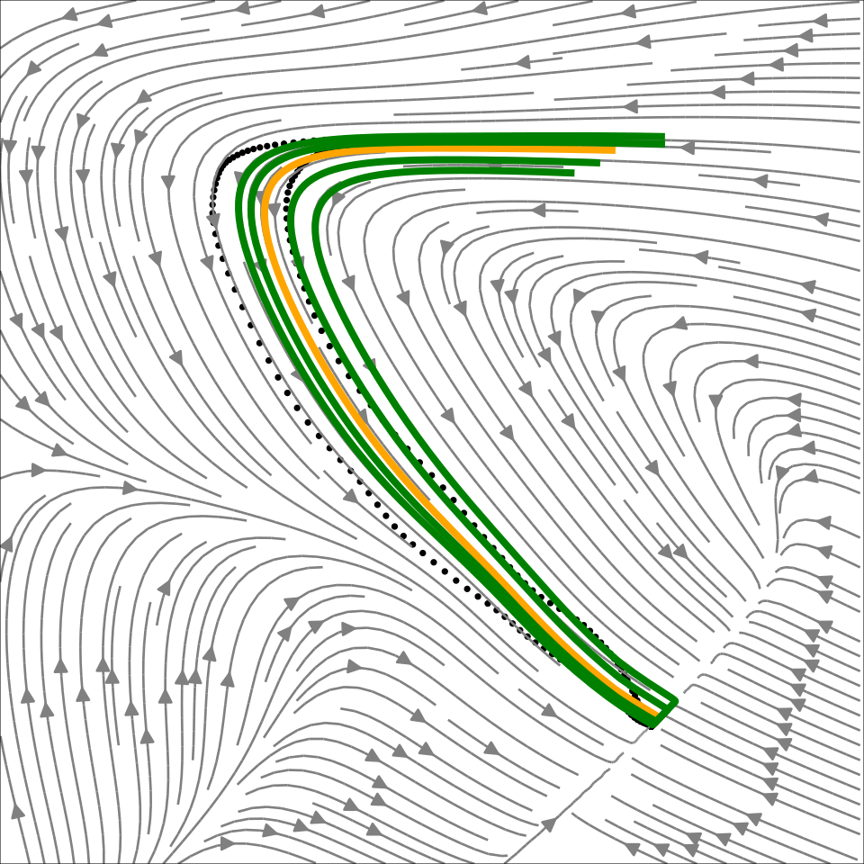
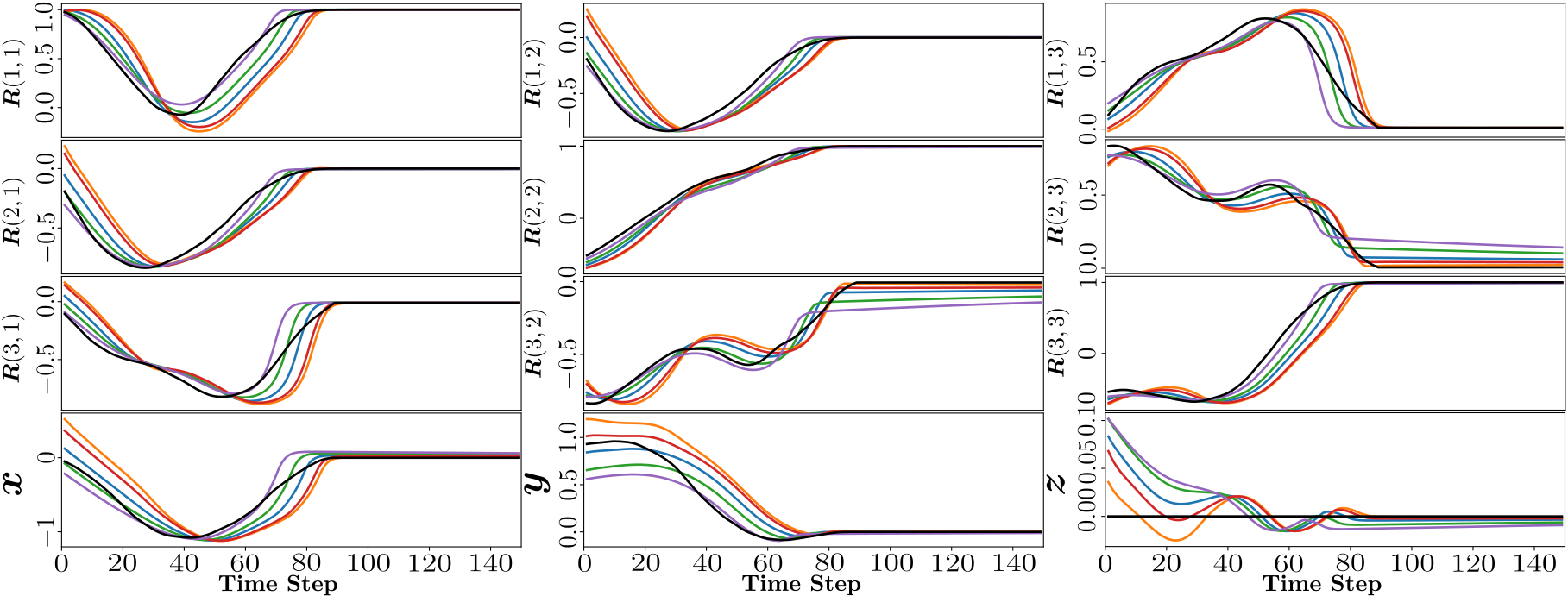
Synthetic full-pose trajectories combine different LASA shapes for position and orientation. Quaternion-derived rotations are mapped to the Lie algebra, producing a six-coordinate state whose learned latent trajectories are visualized.
Original figure
Figure 10: The background depicts the contours of the latent vector field, green and yellow curves depict the path integrals, and black dots represent demonstration in latent space.
Original figure
Figure 11: Time series of demonstrations and path integrals in ℝ3×𝒮​𝒪​(3)\mathbb{R}^{3}\times\mathcal{SO}(3)

A.6.2 Learning human motion

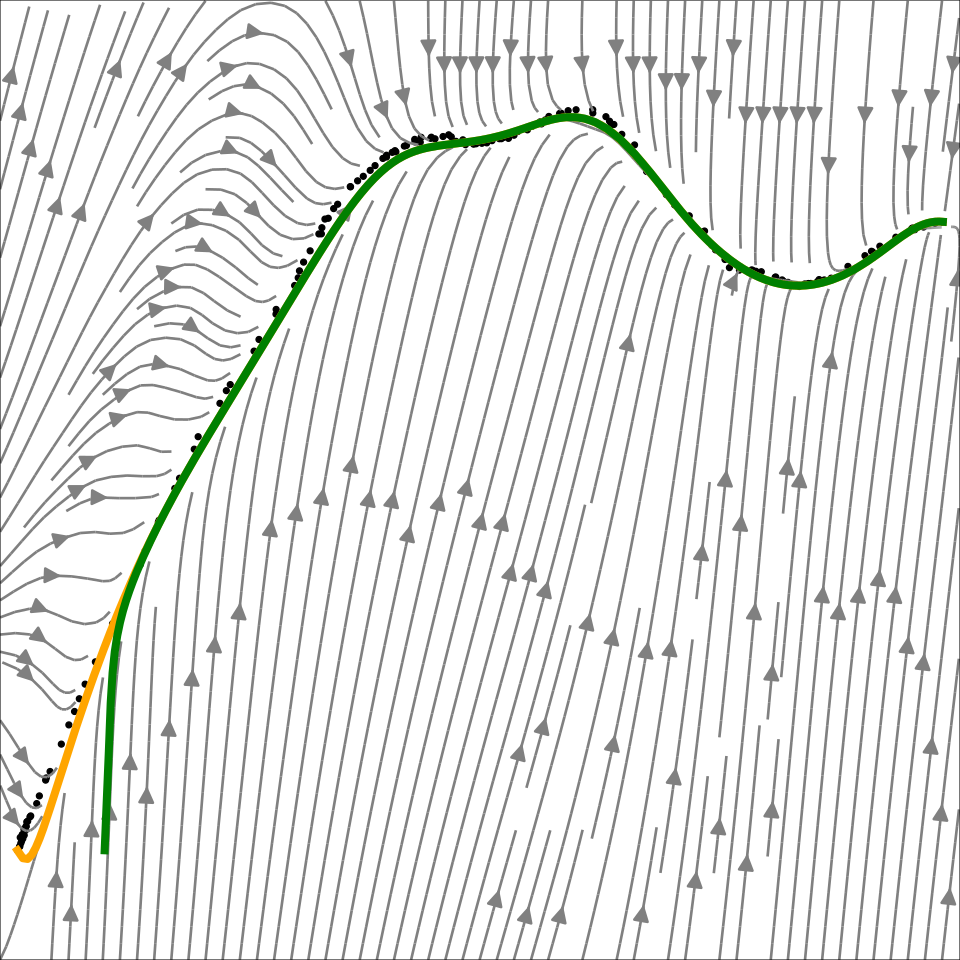
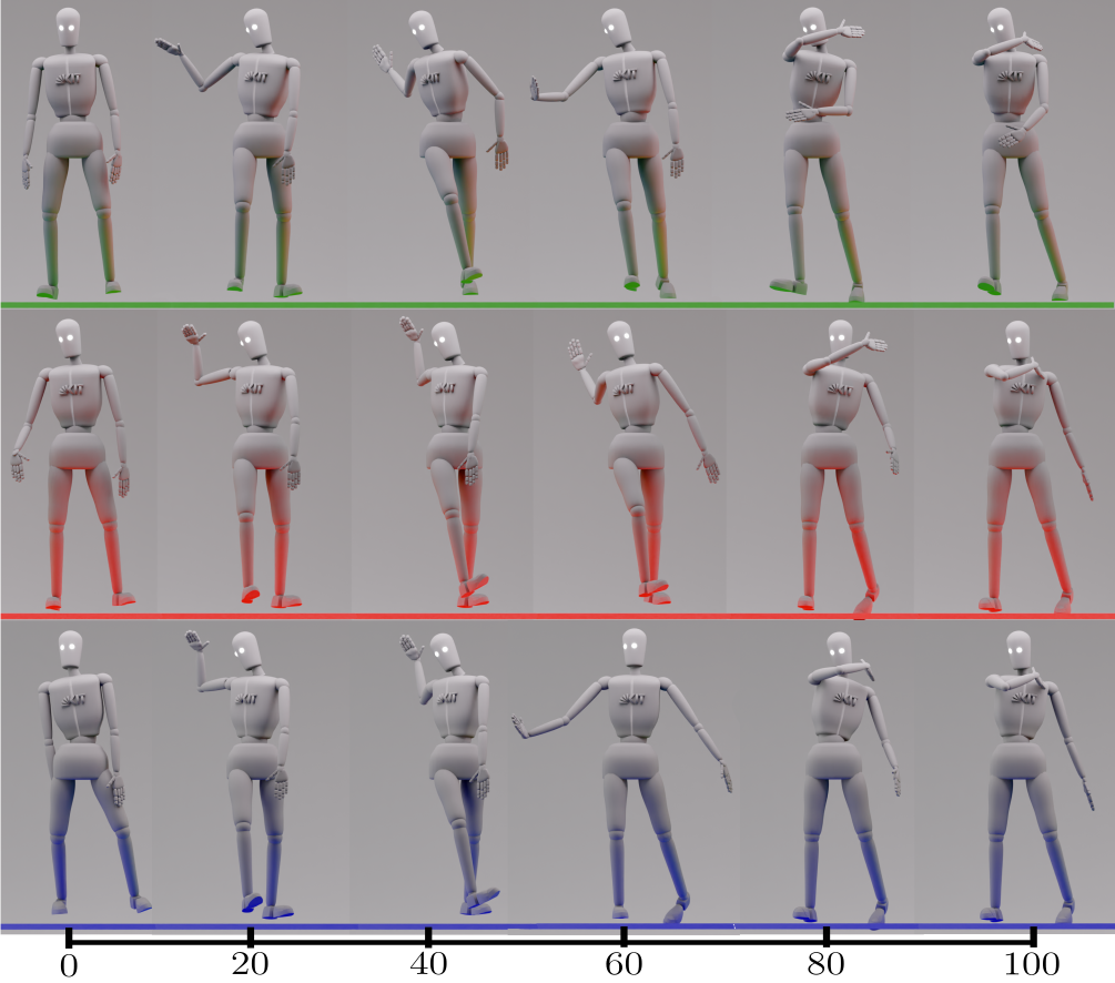
A tennis forehand from the KIT motion dataset is represented by 44 joint coordinates and compressed to two latent dimensions. Generated human-dummy motions illustrate reproduction and extrapolation from different starts.
Original figure
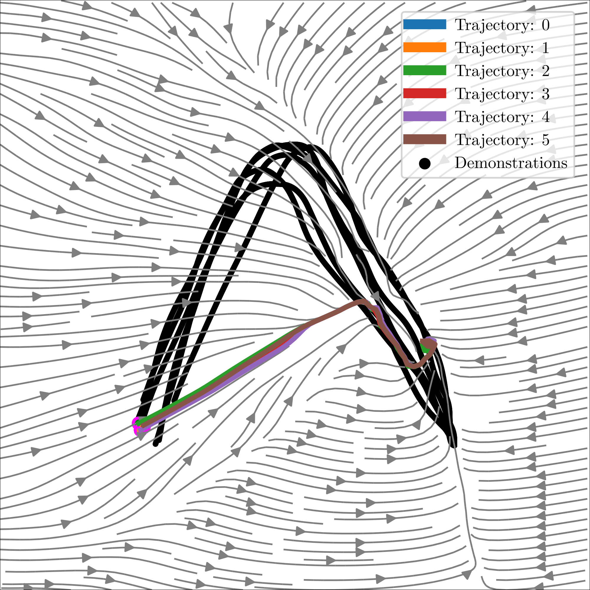
Figure 12: The background depicts the contours of the latent vector field, green and yellow curves depict the path integrals, and black dots represent demonstration in latent space.
Refer to caption
Figure 13: Generated Human Motion with NCDS: The upper row depicts the progressive evolution of the demonstration motion from left to right. Meanwhile, the middle and bottom rows illustrate the motions generated by NCDS when the initial point is respectively distant from and coincident with the initial point of the demonstration.

A.6.3 Quantitative results

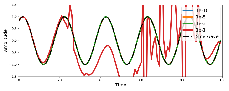
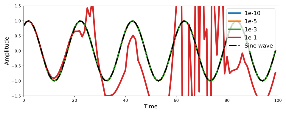
Larger contraction margins reduce expressiveness in the reported ablation. Unconstrained matrix, MLP, and neural-ODE baselines fit observed regions but lack the same observed stability. Integration tolerances and activations affect behavior. Reported single-step timings are 40.9 ms for direct eight-dimensional modeling, 20.2 ms with latent modeling, and 121.0 ms for 44-dimensional latent modeling.
Refer to caption
(a) ϵ=10−4\epsilon=10^{-4}
Refer to caption
(b) ϵ=10−2\epsilon=10^{-2}
Refer to caption
(c) ϵ=10−1\epsilon=10^{-1}
Refer to caption
(d) ϵ=10\epsilon=10
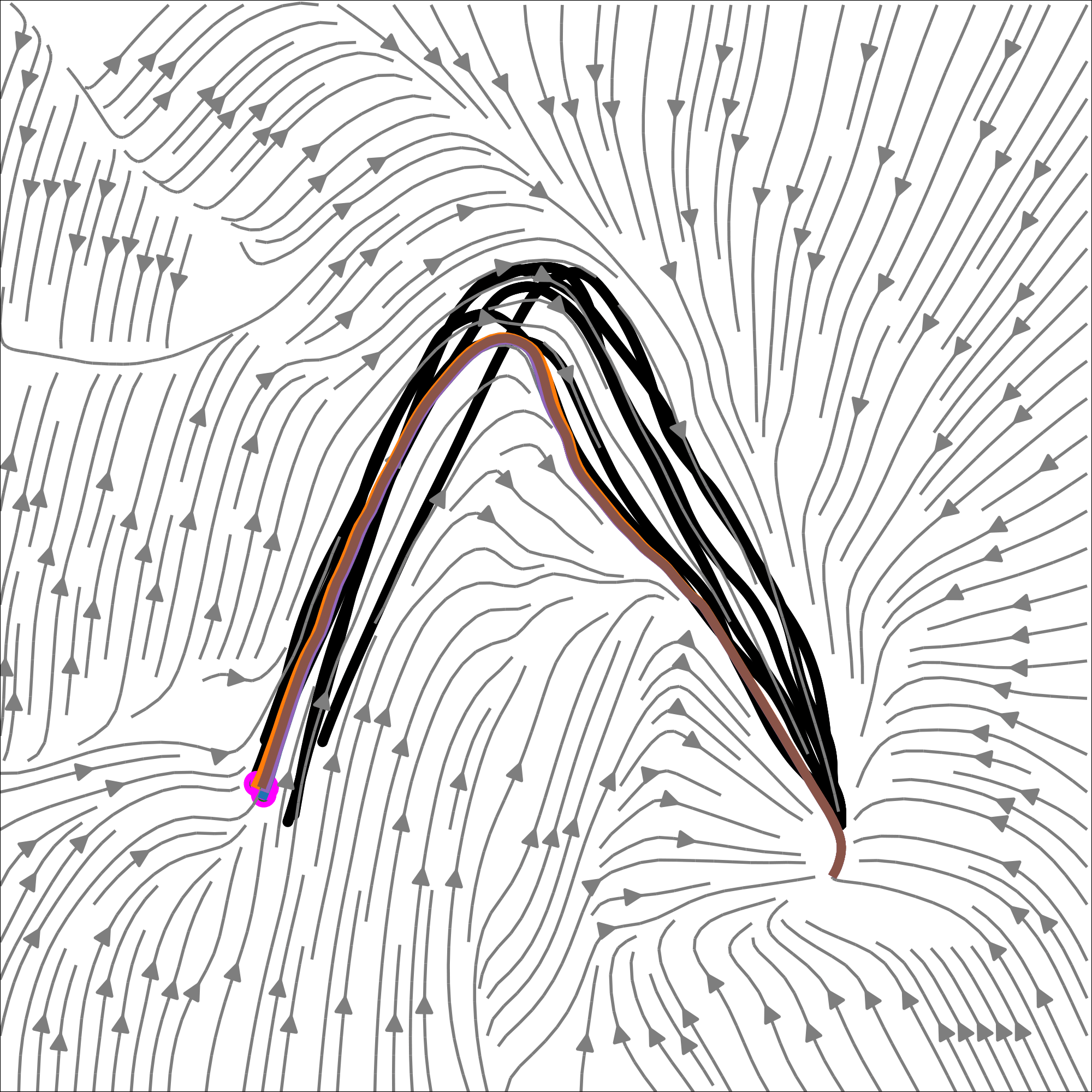
Figure 14: Path integrals generated by NCDS trained using different regularization term ϵ\epsilon.
Refer to caption
(a) Contractive
Refer to caption
(b) Unconstrained
Original figure
(c) MLP
Original figure
(d) Neural ODE
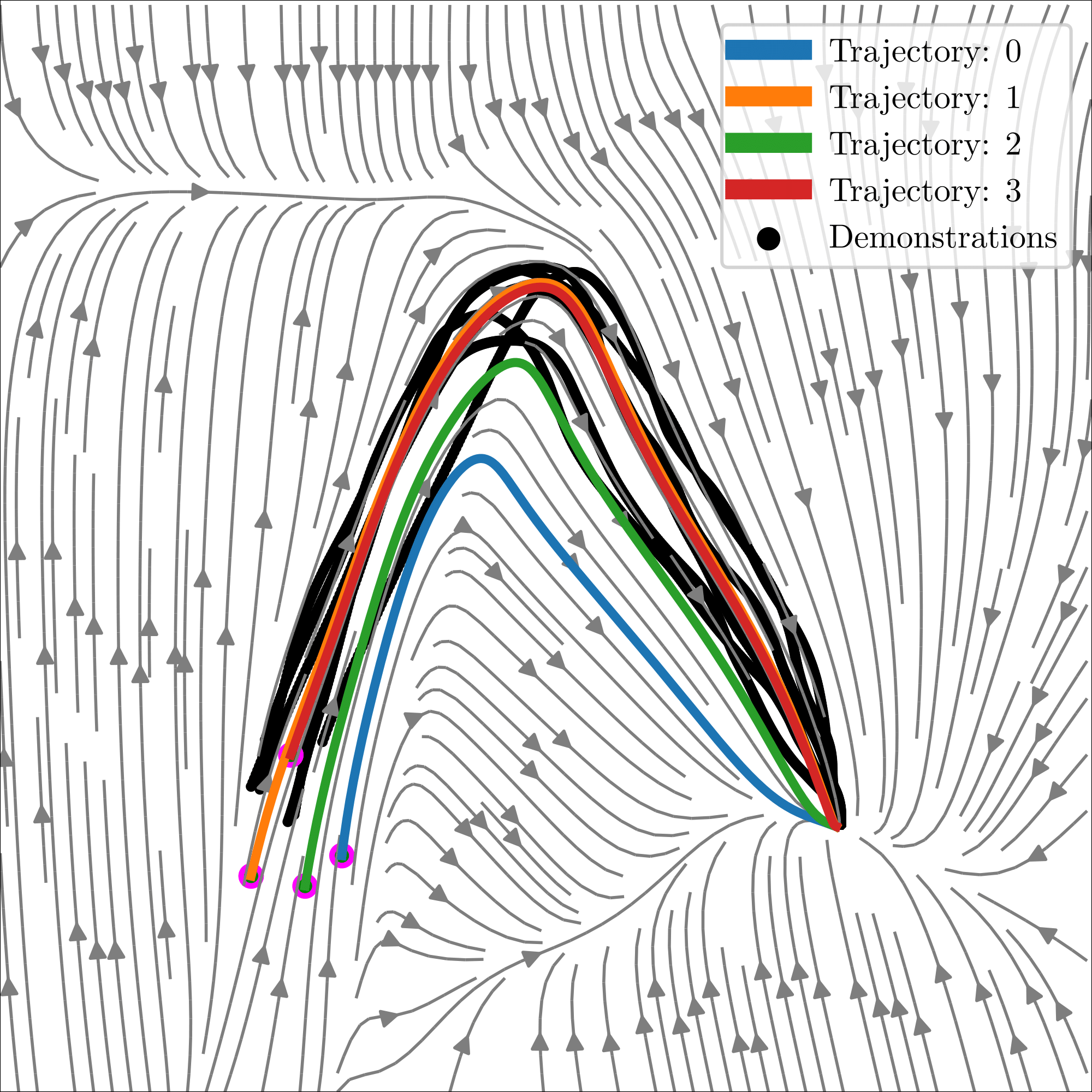
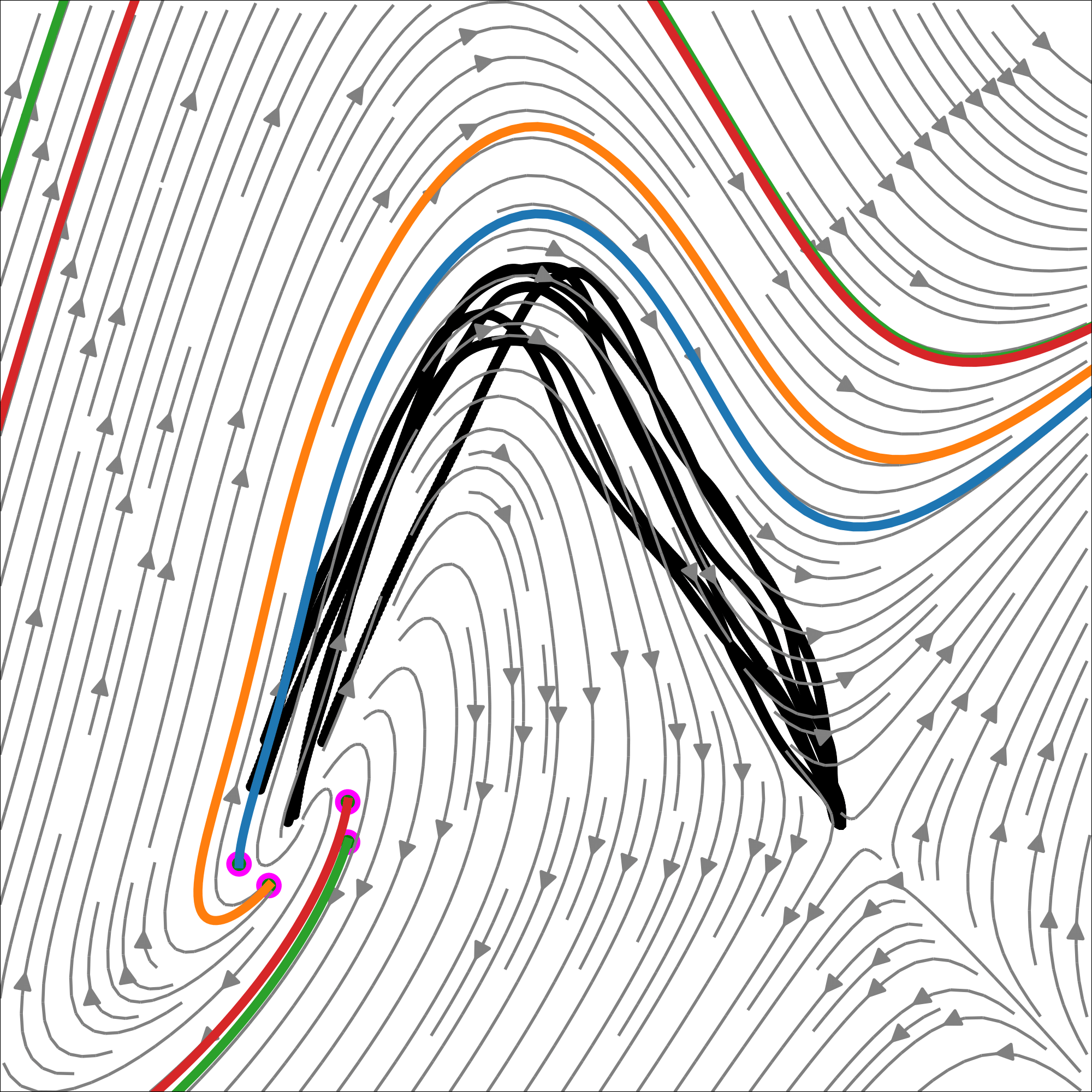
Figure 15: Path integrals generated under the Neural Contractive Dynamical Systems (NCDS) setting, along with baseline comparisons using Multilayer Perceptron (MLP) and Neural Ordinary Differential Equation (NeuralODE) models.
Original figure
(a) Comparison among different absolute tolerance values
Original figure
(b) Comparison among different relative tolerance values
Original figure
(c) Comparison among different integration time steps
Original figure
(d) Comparison among different integration methods
Figure 16: Evaluation of the integrator
Refer to caption
(a) Tanh
Refer to caption
(b) Softplus
Refer to caption
(c) Sigmoid
Figure 17: Path integrals generated by NCDS trained using different activation functions.
Input. Dim 2D 8D
time (ms) 1.23 40.9
Learning the vector field directly in the input space.
Input. Dim 3D 8D 44D
time (ms) 10.6 20.2 121.0
Learning the vector field in the latent space (full pipeline).
Table 2: Average execution time (in milliseconds) of a single integration step

A.6.4 Comparisons

Baseline implementations are tuned for reconstruction: flow architectures vary in depth and coupling structure, while SEDS uses Gaussian components. The comparison assesses accuracy and general stability because the methods offer different stability properties.

A.6.5 Synthetic LASA

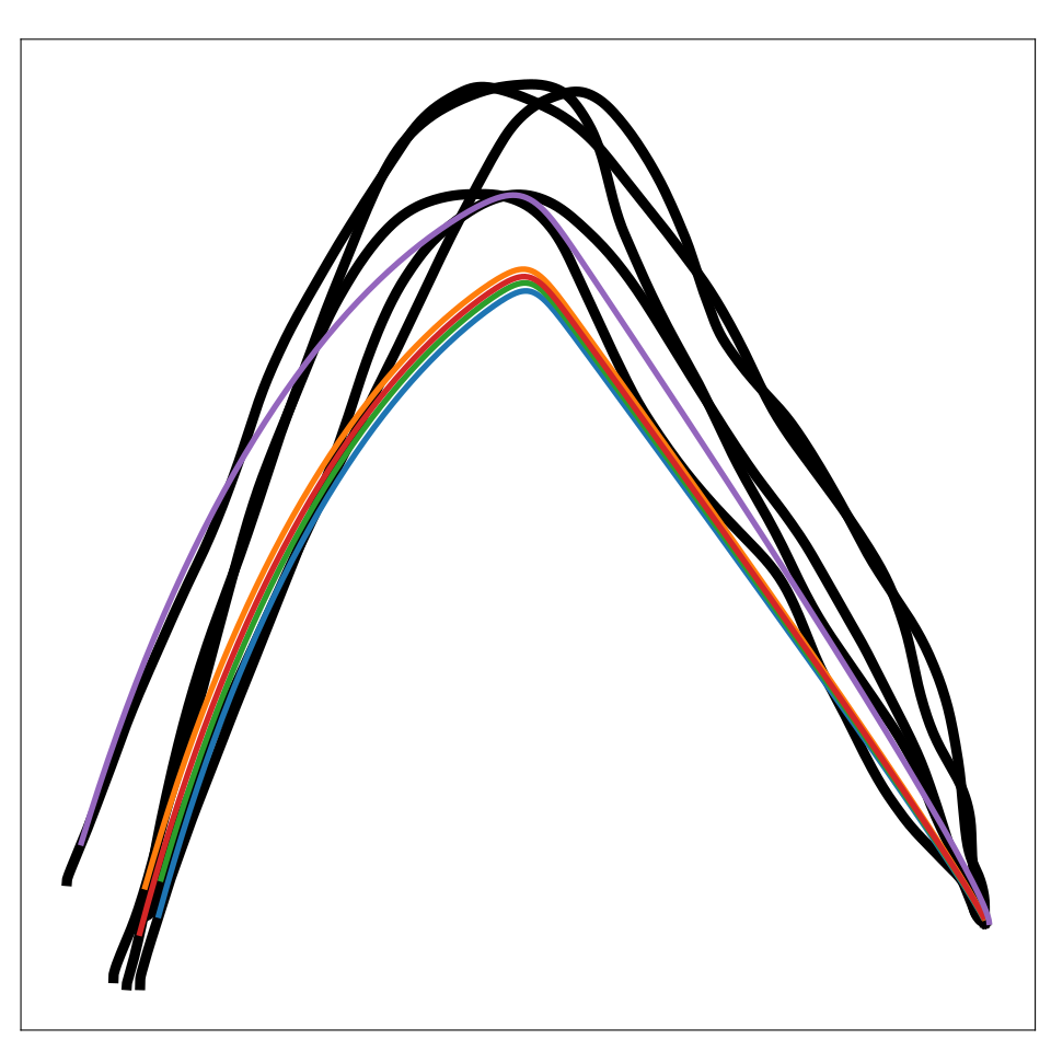
The synthetic benchmark grows from two to eight dimensions by concatenating distinct handwriting motions. Baseline capacity is increased and selected from multiple configurations; NCDS keeps two-dimensional latent dynamics and adds the VAE. Its advantage emerges most clearly in the eight-dimensional case.
Original figure
(a) NCDS
Original figure
(b) SEDS
Original figure
(c) EF
Original figure
(d) IF
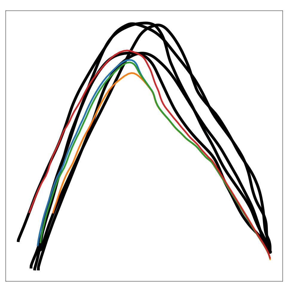
Figure 18: Path integrals generated using different approaches for the two-dimensional LASA problem. All methods provide similar reconstructions.
Original figure
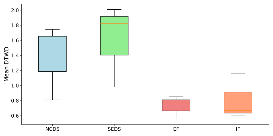
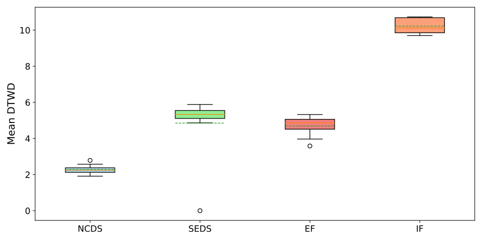
Figure 19: Average dynamic time warping distance between path integrals and the demonstrations for the two-dimensional LASA problem.
Original figure
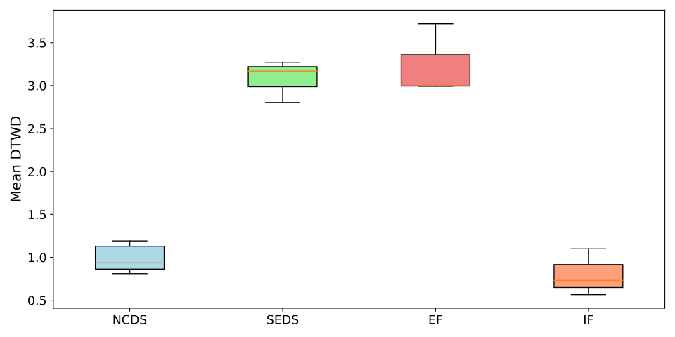
Figure 20: Average dynamic time warping distance between path integrals and the demonstrations for the four-dimensional LASA problem.
Equation 17
𝒟=[xA​n​g​l​e,yA​n​g​l​e,xL​i​n​e,yL​i​n​e,xS​i​n​e,yS​i​n​e,xJ​S​h​a​p​e,yJ​S​h​a​p​e]∈ℝT×8.\mathcal{D}=[x_{Angle},y_{Angle},x_{Line},y_{Line},x_{Sine},y_{Sine},x_{JShape},y_{JShape}]\in\mathbb{R}^{T\times 8}. (17)
Original figure
Figure 21: Average dynamic time warping distance between 5 trajectories constructed with different methods and demonstration trajectories

A.6.6 Joint space dynamics

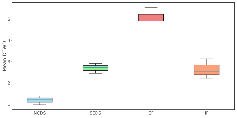
Seven-dimensional joint trajectories provide a Euclidean comparison compatible with all baselines. NCDS has the best reported reconstruction score; accompanying robot reproductions are simulated. The retained literature table distinguishes prior contraction methods and their comparison baselines.
Original figure
Figure 22: Average dynamic time warping distance between path integrals and the demonstrations for the 77-dimensional Joint space problem.
Paper title Abbr. Compared against Year
Safe Control with Learned Certificates: A Survey of Neural Lyapunov, Barrier, and Contraction methods 2022
Learning Contraction Policies from Offline Data MPC (ILQR), RL (CQL) 2022
Neural Contraction Metrics for Robust Estimation and Control: A Convex Optimization Approach NCM CV-STEM, LQR 2021
Learning Stabilizable Nonlinear Dynamics with Contraction-Based Regularization CCM-R 2021
Learning Certified Control Using Contraction Metric C3M SoS (Sum-of-Squares programming), MPC, RL (PPO) 2020
Learning position and orientation dynamics from demonstrations via contraction analysis CDSP SEDS, CLF-DM (Control Lyapunov Function-based Dynamic Movements), Tau-SEDS, NIVF (neurally imprinted vector fields) 2019
Learning Stable Dynamical Systems using Contraction Theory C-GMR SEDS 2017
Learning Contracting Vector Fields For Stable Imitation Learning CVF DMP, SEDS and CLF-DM 2017
Learning Partially Contracting Dynamical Systems from Demonstrations CDSP (only position) DMP, CLF-DM 2017
Table 3: The present state-of-the-art literature pertaining to the learning of contractive dynamical systems.
Concept demonstration

Open image ↗