Overview
The complete paper and implementation appendix are condensed below. All six numbered figures, including every sample grid, eight tables with all six ablation panels, and displayed equations are preserved. The original teaser is reunited with its caption, and omitted ablation-panel descriptions are restored from the PDF.
| T2V (base) | |
|---|---|
| Input | |
| Spatial window | |
| Spatiotermporal window | |
| Training steps | 250000 |
| Batch size | 512 |
| lr schedule | Constant |
| Optimizer | Adafactor |
| lr | 0.00005 |
At a glance
W.A.L.T uses a causal image/video autoencoder and a transformer with spatial and spatiotemporal attention windows for latent diffusion. Shared visual latents permit joint training on images and videos while temporal compression reduces sequence length. Academic benchmarks test image generation, action-conditioned video generation, and frame prediction; a much larger three-stage system generates text-conditioned 512×896 videos at eight frames per second. Classifier-free guidance is omitted in the main controlled benchmarks but used for the text-to-video results.
1 Introduction
Full attention becomes expensive as video sequences grow. Per-frame image latents allow reuse of image data but retain a long temporal sequence; conventional video compression can complicate image/video sharing. W.A.L.T addresses both with an independently encoded first frame and alternating attention patterns. This paper’s contributions are the unified continuous latent representation, an efficient transformer denoiser, controlled benchmark comparisons, and a large text-to-video cascade. Its state-of-the-art claims refer to the systems evaluated in this 2023 source.
2 Related Work
Video Diffusion Models.
Video diffusion can operate in pixels or compressed latents. Inflating pretrained image networks with temporal layers is convenient but often retains per-frame compression. W.A.L.T instead jointly learns an image-compatible spatiotemporal representation and uses it for both data types.
Transformers for Generative Modeling.
Transformers have been used for adversarial, autoregressive, parallel-token, and diffusion generation. This work uses diffusion denoising over continuous video latents, avoiding token-by-token generation within a clip. Longer videos still require repeated clip generation.
3 Background
Training corrupts real samples with Gaussian noise and learns the reverse process. All experiments predict the velocity-style target combining clean data and noise. The autoencoder compresses space and time, and its decoder reconstructs pixels. Although motivated by vector-quantized autoencoders, this model uses continuous latents without a codebook. Adversarial and perceptual reconstruction losses improve decoded quality.
Equations 1–2
| (1) |
| (2) |
4 W.A.L.T
4.1 Learning Visual Tokens
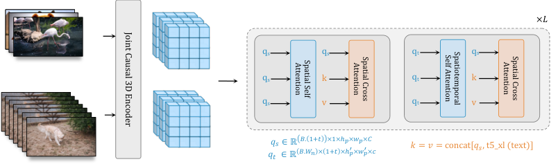
A causal three-dimensional convolutional encoder processes each frame using only its present and past context. The first frame can therefore be encoded independently, so an image is simply a one-frame input. The remaining frames are temporally compressed. The MAGVIT-v2-style encoder/decoder is adapted to quantization-free latents; training batches can contain video clips and stacks of independent images.
4.2 Learning to Generate Images and Videos
Each latent frame is patchified and given learned spatial and temporal positions, with additional relative positions. Spatial attention covers tokens within one latent frame. Spatiotemporal attention spans time within a smaller spatial window; independent-image inputs use an identity mask in this layer. Alternation models spatial detail and video dynamics at lower memory cost than global space-time attention. Joint video encoding reduces a source of per-frame flicker, but does not prove that every generated sequence is artifact-free.
4.3 Conditional Generation
Text conditions use cross-attention; joint image/video training applies it in spatial layers. Adaptive layer normalization modulates features with condition and diffusion-time embeddings. AdaLN-LoRA shares most conditioning parameters and adds a low-rank per-layer correction: in the cited one-billion-parameter transformer example, rank two reduces these extra parameters from 475 million to 12 million. Self-conditioning sometimes predicts a clean latent estimate and feeds a stopped-gradient copy into a second denoising pass, trading additional training computation for quality.
Equation 3
| (3) |
| Method | K600 FVD | UCF FVD | params. | steps |
| TrIVD-GAN-FP [51] | 25.7±0.7 | – | – | 1 |
| Video Diffusion [36] | 16.2±0.3 | – | 1.1B | 256 |
| RIN [41] | 10.8 | – | 411M | 1000 |
| TATS [23] | – | 332±18 | 321M | 1024 |
| Phenaki [74] | 36.4±0.2 | – | 227M | 48 |
| MAGVIT [81] | 9.9±0.3 | 76±2 | 306M | 12 |
| MAGVITv2 [82] | 4.3±0.1 | 58±2 | 307M | 24 |
| W.A.L.T-L Ours | 3.3±0.0 | 46±2 | 313M | 50 |
| W.A.L.T-XL Ours | – | 36±2 | 460M | 50 |
4.4 Autoregressive Generation
Frame-prediction training conditions on one latent frame for image animation or two for video continuation, with a mask identifying supplied context. At inference, repeated conditional generation extends the clip using classifier-free guidance. This supports longer sequences but does not establish indefinite temporal consistency.
4.5 Video Super Resolution
A base model produces low-resolution video and two super-resolution models each double spatial resolution. The refiners receive upscaled latents and noise augmentation, reducing their mismatch between clean training inputs and imperfect generated inputs. The base model is trained square, then fine-tuned for a 128×224 landscape frame through positional-embedding interpolation; later stages reach 512×896.
| Method | Cost (IterBS) | FID | IS | params. | steps |
|---|---|---|---|---|---|
| BigGAN-deep [6] | - | 6.95 | 171.4 | 160M | 1 |
| LDM-4 [61] | 178k1200 | 10.56 | 103.5 | 400M | 250 |
| DiT-XL/2 [53] | 7000k256 | 9.62 | 121.5 | 675M | 250 |
| ADM [16] | - | 7.49 | 127.5 | 608M | 2000 |
| MDT [22] | 6500k256 | 6.23 | 143.0 | 676M | 250 |
| MaskDiT [87] | 1200k1024 | 5.69 | 178.0 | 736M | 40 |
| RIN [41] | 600k1024 | 3.42 | 182.0 | 410M | 1000 |
| simple diffusion [38] | 500K2048 | 2.77 | 211.8 | 2B | 512 |
| VDM++ [45] | - | 2.40 | 225.3 | 2B | 512 |
| W.A.L.T-L Ours | 437k1024 | 2.56 | 215.1 | 460M | 50 |
5 Experiments
The evaluation separates controlled academic datasets from the larger, heterogeneous text-to-video training setting.
5.1 Visual Generation
For class-conditioned UCF-101, W.A.L.T-XL reports FVD 36±2 with 460 million parameters and 50 DDIM steps, versus MAGVIT-v2’s 58±2. For Kinetics-600 prediction from five observed frames, W.A.L.T-L reports FVD 3.3 versus 4.3 for MAGVIT-v2. ImageNet evaluation generates 50,000 images at 256×256: W.A.L.T reports FID 2.56 and Inception Score 215.1 without guidance. VDM++ has a lower FID of 2.40, with a larger reported parameter count. These distributional metrics compare benchmark samples; they do not directly measure physical correctness or complete text alignment.
| FVD | IS | params | |
|---|---|---|---|
| 2 | 60.7 | 87.2 | 313 M |
| 4 | 56.6 | 87.3 | 314 M |
| 16 | 55.5 | 88.0 | 316 M |
| 64 | 54.4 | 87.9 | 324 M |
| 256 | 52.5 | 88.5 | 357 M |
5.2 Ablation Studies
UCF-101 ablations use 35,000 training steps. Smaller patches substantially improve FVD. Local temporal windows provide comparable quality with up to roughly twice the reported steps per second of full attention. Self-conditioning improves over none, although the displayed 0.6 rate slightly beats 0.9 on FVD. Larger AdaLN-LoRA ranks improve quality at increased parameter cost. A parameter-matched comparison favors different configurations on different measures: the larger shared-conditioning backbone has lower training loss but slightly worse FVD. Zero terminal signal-to-noise ratio prevents residual clean-signal leakage during the highest-noise training step and improves generation. Increasing latent channels improves reconstruction, but generation is nonmonotonic: the shown channel-16 model has better FVD than channel eight, while channel 32 worsens it. The authors retain eight as a robust default across tasks. Thus the original “higher is better” panel captions should be read alongside the actual metric columns.
| Model | AdaLN | FVD | IS | params. | final loss |
|---|---|---|---|---|---|
| L | separate | 34.6 | 90.2 | 458M | 0.274 |
| XL | LoRA-2 | 36.7 | 89.4 | 460M | 0.268 |
5.3 Text-to-video
Text-to-video training uses approximately 970 million image-text pairs and 89 million video-text pairs from public internet and internal sources. The base model has three billion parameters, followed by approximately 1.3 billion- and 419 million-parameter refiners. All text-to-video results use classifier-free guidance. These data and model scales differ substantially from the controlled benchmark experiments.
5.3.1 Quantitative Evaluation
Under the zero-shot UCF-101 text protocol, adding images to a 419-million-parameter model improves FVD from 598.8 to 344.5; scaling the jointly trained base to three billion parameters yields 258.1 and Inception Score 35.1. The listed PYoCo comparison has FVD 355.2 but a higher Inception Score, 47.8. Training data and text encoders vary across systems, so this is a system-level comparison rather than a controlled architecture comparison. W.A.L.T uses T5-XL; the source suggests stronger text conditioning as one possible explanation for the score difference.
| Method | IS () | FVD () |
|---|---|---|
| CogVideo (Chinese) [37] | 23.6 | 751.3 |
| CogVideo (English) [37] | 25.3 | 701.6 |
| MagicVideo [88] | - | 699.0 |
| Make-A-Video [66] | 33.0 | 367.2 |
| Video LDM [4] | 33.5 | 550.6 |
| PYoCo [24] | 47.8 | 355.2 |
| W.A.L.T (Ours) 419M (video only) | 26.8 | 598.8 |
| W.A.L.T (Ours) 419M (video + image) | 31.7 | 344.5 |
| W.A.L.T (Ours) 3B (video + image) | 35.1 | 258.1 |
5.3.2 Qualitative Results
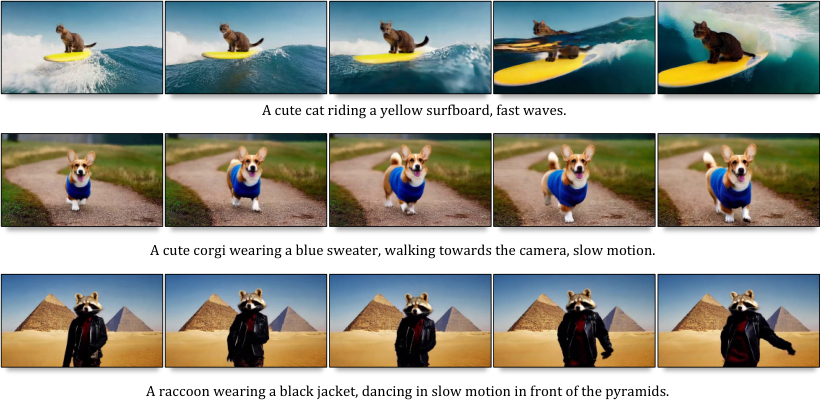
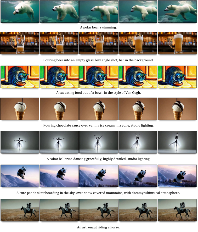
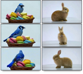
The retained examples illustrate text-conditioned clips, image animation, and camera movement around an object. Figure 4 shows a 5.1-second continuation example. Full temporal behavior is better assessed in the accompanying videos than from selected still frames.
6 Conclusion
A shared causal visual representation and windowed transformer make joint image/video latent diffusion practical and competitive in the reported tests. Remaining practical limits include the large data and model requirements, cascaded inference, incomplete standardization of text-to-video evaluation, and lack of direct guarantees for physical realism or long-horizon consistency.
Acknowledgements
The authors acknowledge the listed colleagues for feedback and discussions.
Appendix A Implementation Details
The appendix supplies training and inference settings for the autoencoders, denoisers, and refiners. Final UCF-101 results use 60,000 steps; ablations use 35,000. The usual compression factors are eight spatially and four temporally, turning a 17-frame clip into five latent frames. Aspect-ratio fine-tuning changes spatial windows and interpolates absolute and relative positions. To continue a generated 17-frame clip, the last five decoded frames are encoded into two context latents for the next prediction. UCF class prompts are adapted from prior evaluation wording. The main text says patch size two for the final refiner, while Table 8 lists four; both source descriptions remain available rather than being silently reconciled.
Appendix B Additional Results
B.1 Image Generation
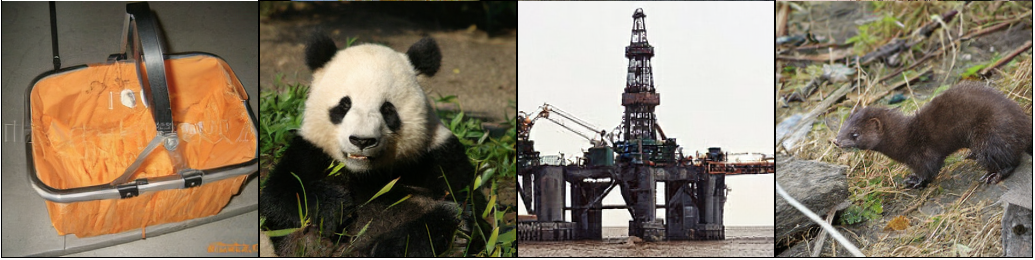
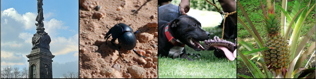
The guided ImageNet comparison uses a power-cosine guidance schedule because ordinary guidance showed little benefit. W.A.L.T reports FID 2.40 and Inception Score 290.5: the latter leads the displayed comparisons, while several alternatives have lower FID. Both rows of generated samples are retained.
| Method | Cost (IterBS) | FID | IS | Params. | Steps |
|---|---|---|---|---|---|
| LDM-4 [61] | 178k1200 | 3.60 | 247.7 | 400M | 250 |
| DiT-XL/2 [53] | 7000k256 | 2.27 | 278.2 | 675M | 250 |
| ADM [16] | - | 3.94 | 215.8 | 608M | 2000 |
| MDT [22] | 6500k256 | 1.79 | 283.0 | 676M | 250 |
| MaskDiT [87] | 1200k1024 | 2.28 | 276.6 | 736M | 40 |
| simple diffusion [38] | 500K2048 | 2.44 | 256.3 | 2B | 512 |
| VDM++ [45] | - | 2.12 | 267.7 | 2B | 512 |
| W.A.L.T-L Ours | 437k1024 | 2.40 | 290.5 | 460M | 50 |
| ImageNet | UCF-101 | K600 | T2V (base) | T2V (2) | T2V (22) | |
| First Stage | ||||||
| Input | ||||||
| 8, - | 8, 4 | 8, 4 | 8, 4 | 8, 4 | 8, 4 | |
| Channels | 128 | 128 | 128 | 128 | 128 | 128 |
| Channel multiplier | 1,1,2,4 | 1, 2, 2, 4 | 1, 2, 2, 4 | 1, 2, 2, 4 | 1, 2, 2, 4 | 1, 2, 2, 4 |
| Training duration | 270 epochs | 2000 epochs | 270000 steps | 1000000 steps | 1000000 steps | 1000000 steps |
| Batch size | 256 | 256 | 256 | 256 | 256 | 256 |
| lr schedule | Cosine | Cosine | Cosine | Cosine | Cosine | Cosine |
| Optimizer | Adam | Adam | Adam | Adam | Adam | Adam |
| Second Stage | ||||||
| Input | ||||||
| Layers | 24 | 28 | 24 | 52 | 40 | 24 |
| Hidden size | 1024 | 1152 | 1024 | 9216 | 1408 | 1024 |
| Heads | 16 | 16 | 16 | 16 | 16 | 16 |
| Training duration | 350 epochs | 60000 steps | 360 epochs | 550000 steps | 675000 steps | 275000 steps |
| Batch size | 1024 | 256 | 512 | 512 | 512 | 512 |
| lr schedule | Cosine | Cosine | Cosine | Cosine | Cosine | Cosine |
| Optimizer | AdamW | AdamW | AdamW | Adafactor | Adafactor | Adafactor |
| lr | 0.0005 | 0.0005 | 0.0005 | 0.0002 | 0.0005 | 0.0005 |
| EMA | ✗ | ✗ | ✗ | |||
| Patch size | 1 | 1 | 1 | 1 | 2 | 4 |
| AdaLN-LoRA | ✗ | 2 | 2 | 2 | 2 | 2 |
| Diffusion | ||||||
| Diffusion Steps | 1000 | 1000 | 1000 | 1000 | 1000 | 1000 |
| Noise schedule | Linear | Linear | Linear | Linear | Linear | Linear |
| 0.0001 | 0.0001 | 0.0001 | 0.0001 | 0.0001 | 0.0001 | |
| 0.02 | 0.02 | 0.02 | 0.02 | 0.02 | 0.02 | |
| Sampler | DDIM | DDIM | DDIM | DDIM | DDIM | DDIM |
| Sampling steps | 50 | 50 | 50 | 50 | 50 | 50 |
| Guidance | ✗ | ✗ | ✗ |
B.2 Video Generation
All three Kinetics prediction panels preserve the ground-truth and generated sequences, with unobserved ground-truth frames shaded. These are qualitative examples rather than additional aggregate metrics.



B.3 Image-to-Video
Conditioning on a single latent image lets the model animate an image-generator output. The appendix points to project videos for this qualitative setting rather than reporting a separate image-to-video benchmark.