At a glance
When can one compact relational neural policy solve a planning problem across different numbers of objects? This paper constructs policies from goal-regression search and relates their required depth and relation arity to strong optimal serializability (SOS) width. Small fixed width permits a fixed breadth of relations; planning depth can still grow with the problem. A suitable regression-rule selector can reduce the required computation further.
These are representation and compilation results for discrete, deterministic planning classes. They do not guarantee that training discovers the constructed policy, that a fixed architecture solves general planning, or that all practical tasks have small width. Experiments illustrate the depth dependence in three small domains.
1 Introduction
A policy shared across instances needs to handle a varying number of objects while preserving the reasoning needed to choose actions. The analysis connects classical planning, regression search, and relational circuits instead of treating network size as an arbitrary hyperparameter. General propositional planning remains PSPACE-complete (Bylander, 1994); restricted domain and goal classes can nevertheless have compact policies.
The central distinction is between breadth—the maximum arity of a relation represented by the network—and depth, the number of computational layers per policy decision. Breadth is not the ordinary hidden-channel width, and bounded arity does not mean a constant total number of tensor entries as the object count grows.
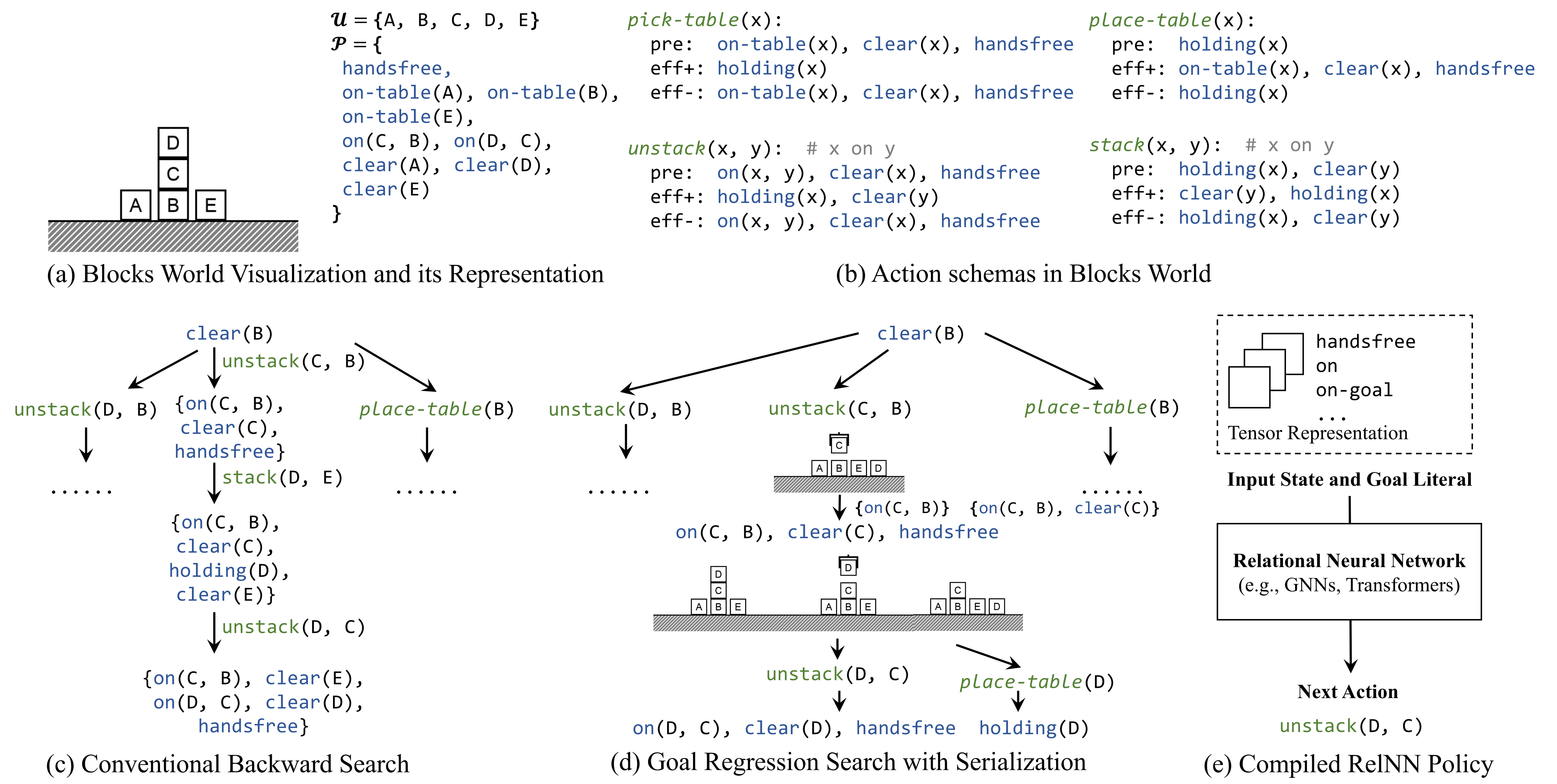
2 Preliminaries: Planning Domain and Problem
The setting is classical deterministic planning over a fixed set of objects and Boolean ground atoms. A state lists true atoms; a STRIPS action has preconditions plus add and delete effects. The retained transition formula specifies applicability and the next state. A goal-conditioned policy repeatedly chooses actions until the goal holds.
The analysis primarily uses a single-atom goal. A conjunction can be compiled into a goal-achieve action, but its preconditions can increase the relevant width. Object creation, uncertain dynamics, and continuous control are outside these formal assumptions.
Equation
3 Goal Regression Search and Width
Plain backward search starts from the desired goal set, chooses a final action that achieves a goal without deleting another, and regresses to its preconditions. A goal stack prevents recursive cycles. Algorithm 1 retains the exact procedure. Its cost depends on both planning horizon and intermediate goal-set size and is exponential in the general case.
3.1 Serialized Goal Regression Search
Serialized goal regression search (S-GRS) commits to an order for achieving an action’s preconditions. When solving the next precondition, it preserves external constraints and previously achieved preconditions; an admissible final action must not delete those constraints. The retained rules show this explicitly for clearing a block.
Algorithm 2 keeps a shortest local subplan. In general this loses completeness or optimality because different ways to achieve a subgoal can leave different states. Appendix A.1’s exhaustive variant tracks those alternatives; the faster main algorithm has guarantees only under the stated serializability conditions.
Equations
3.2 Serialization of Goal Regression Rules
Optimal serializability requires optimal prefix plans to extend through each ordered precondition and finally to an optimal plan for the goal. The exact definition and Theorem 3.1 are retained. The completeness claim applies to goals reachable through the optimally serializable rules, not arbitrary action orderings or arbitrary planning instances.
Definition 3.1 (Optimal serializability).
A goal regression rule is optimally serializable w.r.t. a state if and only if, for all steps , if and then . Furthermore, , §§ § denotes concatenation of sequences..
3.3 Width of Search Problems
Generalized rules explicitly preserve only selected earlier preconditions. Their width counts those retained constraints plus the external constraint set. Strong optimal serializability adds a crucial requirement: any optimal plan under the selected constraints must still achieve the full relevant prefix. Small syntactic width alone is insufficient.
For SOS width k, Theorem 3.2 bounds search by O(N^(k+1)), where N counts ground atoms, suppressing polynomial action-enumeration factors. Theorem 3.3 connects SOS width k to forward width at most k + 1 and iterated-width search. This is an upper bound; the two widths need not be equal.
Definition 3.2 (Generalized regression rules).
A generalized, optimally-serializable regression rule is , where . Its width is .
Definition 3.3 (Strong optimally-serializable (SOS) width of regression rules).
A generalized regression rule has strong optimally-serializable width w.r.t. state if (a) it is optimally serializable, (b) its width is , and, (c) .
Definition 3.4 (SOS width of problems).
A planning problem has strong optimally-serializable width if there exists a set of strong optimally-serializable width rules w.r.t. , such that S-GRS can solve using only rules in .
Theorem 3.2.
If a problem is of SOS width , it can be solved in time with s-grs, where is the number of atoms. Here we have omitted polynomials related to enumerating all possible actions and their serializations (which are polynomial w.r.t. the number of objects in ).
4 Policy Realization
A relational network receives the state and goal as predicates over objects and predicts an action. Shared parameters allow different object counts, while higher-arity tensors can still be large. The paper gives two constructions: unroll general search, or use a state-dependent rule selector to avoid much of that search.
4.1 Relational Neural Network Background
A RelNN[D, B] has D layers and maximum relation arity B. Hidden feature dimension is assumed bounded, although the number of object tuples grows with instance size. Under this model, bounded-variable first-order logic with counting characterizes representable computations, following Luo et al. and the related logical expressivity results cited in Lemma 4.1.
The lemma’s lower bound separates families of logical functions requiring B versus B − 1 variables. It does not by itself prove that every fixed-breadth network fails on every difficult planning domain.
Lemma 4.1 (Logical expressiveness of relational neural networks (Luo et al., 2022; Cai et al., 1992)).
Let FOCB denote a fragment of first-order logic with at most variables, extended with counting quantifiers of the form , which state that there are at least nodes satisfying formula .
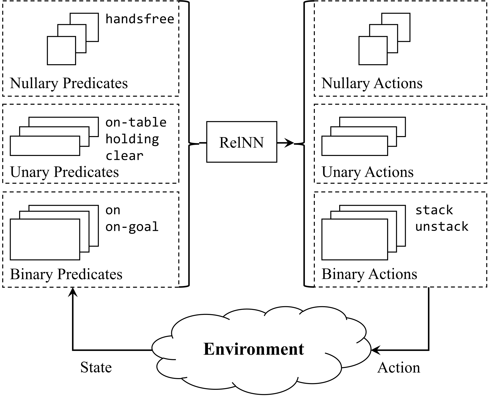
4.2 Compilation of BWD and S-GRS
Unrolling backward search gives depth O(T) and breadth β·k_BWD, where T is the optimal planning horizon, β the maximum predicate arity, and k_BWD the largest regressed goal-set size. The SOS construction reduces breadth to (k + 1)β while retaining O(T) depth.
Thus a domain with constant SOS width can have finite breadth even when the straightforward backward-search encoding does not. Depth may still be unbounded or even exponential in the object count through T. These are constructive upper bounds, not efficient training guarantees.
Theorem 4.1 (Compilation of BWD).
Given a planning problem , let T be the length of the optimal trajectory (the planning horizon), be the maximum number of atoms in the goal set in bwd, and be the maximum arity of atoms in the domain. The backward search algorithm bwd can be compiled into a relational neural network in .
Theorem 4.2 (Compilation of S-GRS).
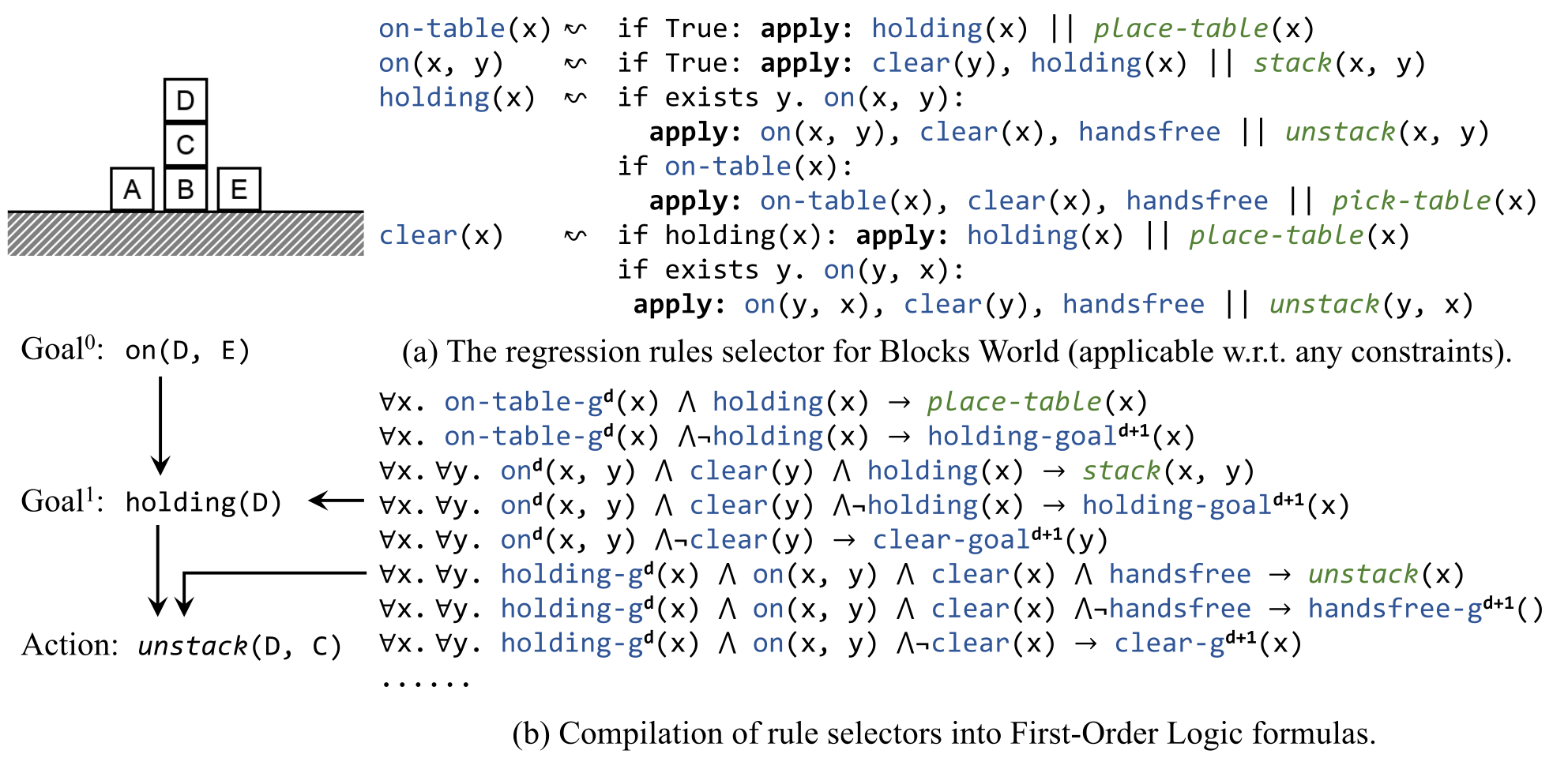
4.3 Compilation of S-GRS with a Regression Rule Selector
A regression-rule selector uses the current state, goal, and constraints to choose an action, an ordering of its preconditions, and bindings for any free variables. In Blocks World, the block directly above the target selects the useful unstack rule. Resource-dependent free-variable choices can make such a selector much harder to express.
Given a selector, the compiled policy traces the first unsatisfied precondition until it reaches an executable action. The exact selector definition, serializability condition, theorem, and lifted policy rules are retained. Selector construction is not automatic: it may require domain knowledge or learning.
Definition 4.1 (RRS Serializability).
A regression rule selector is serializable if and only if the following condition holds for any state , any goal , and any constraint set. Consider the regression rule returned by . If is achievable from , then it can be achieved via the concatenation of the following trajectories: , , , , and .
Equations
Compiling policy neural networks.
Theorem 4.3 gives depth O(d·D_r) and breadth max(B_r, β), with d the regression-tree depth and D_r/B_r the selector’s circuit requirements. The policy must follow a selector that actually yields a plan. A balanced regression tree can reduce depth relative to plan length, but a chain can still require linear depth; a logarithmic reduction is not universal.
Variable iterations of a recurrent layer can handle increasing depth. A derived predicate such as above(x, y) can also shorten inference, but it supplies additional reachability information. Such an encoding shortcut should not be confused with solving the same reasoning problem from the original immediate-neighbor predicates.
Theorem 4.3 (Compilation of S-GRS with a regression rule selector).
Given a regression rule selector select (i.e., the state-constraint condition function ) that can be computed by a relational neural network in , for any planning problem , if , letting be the depth of the regression tree, then there is a RelNN circuit for the problem in , where is the maximum arity of predicates.
Equation
5 Problem Analysis and Results
The domain analysis and Table 1 concern single-atom goals. Blocks World, Logistics, Gripper, Rover, and Elevator have the stated constant-breadth constructions; most still need unbounded depth. Gripper’s constant-depth case assumes direct travel between rooms. The paper classifies Sokoban as unbounded and nonserializable under its analysis; the constructive upper-bound theorems alone are not a general neural-circuit lower-bound proof.
Experiments use Neural Logic Machines with hidden dimension 64, three random seeds, and standard errors. Assembly3 requires selecting a compatible A–B–C chain. With training on ten objects, breadth-two/depth-two networks achieve 100% at 10, 30, and 50 objects; depth one falls from 20% to 2% and 0%.
In the generated Logistics graphs, depth three scores 100%, 30%, and 23%, while depth n/5 + 1 scores 100% at all three sizes. That adaptive depth is manually chosen for the graph generator. For BlocksWorld-Clear, both policies succeed, but depth n/10 + 3 yields average plans of 2.5, 3.1, and 3.5 steps versus 2.9, 10.2, and 15.7 for fixed depth three. Success alone therefore hides a substantial planning-efficiency difference.
|
|
| ||||
| BlocksWorld | ✓ () | Unbounded | ||||
| Logistics | ✓ () | Unbounded | ||||
| Gripper | ✓ () | Constant | ||||
| Rover | ✓ () | Unbounded | ||||
| Elevator | ✓ () | Unbounded | ||||
| Sokoban | ✗ | Unbounded |
| Task | Model | n=10 | n=30 | n=50 |
| As3 | 0.2±0.05 | 0.02±0.01 | 0.0±0.0 | |
| As3 | 1.0±0.0 | 1.0±0.0 | 1.0±0.0 | |
| Log. | 1.0±0.0 | 0.30±0.03 | 0.23±0.05 | |
| Log. | 1.0±0.0 | 1.0±0.0 | 1.0±0.0 | |
| BW | 1.0 / 2.9±0.4 | 1.0 / 10.2±0.45 | 1.0 / 15.7±2.5 | |
| BW | 1.0 / 2.5±0.4 | 1.0 / 3.1±0.5 | 1.0 / 3.5±0.4 |
6 Related Work and Conclusion
The work connects planning width and serialization with hierarchical task networks, hierarchical goal networks, relational expressivity, and algorithmic alignment. It explains why some object-centric problem classes admit compact policies and how constraints or long dependency chains can increase required computation.
The proofs establish existence and circuit bounds within discrete first-order domains. Learning the selector, handling resources, extending to continuous perception and action, and constructing universal multi-domain policies remain separate problems. The small experiments support the predicted depth dependence in their generators rather than general planning competence.
Acknowledgement.
The authors acknowledge reviewer feedback and support from ONR/MURI, the Center for Brains, Minds and Machines, NSF, AFOSR, ARO, MIT–IBM Watson AI Lab, MIT Quest for Intelligence, and Boston Dynamics AI Institute. The stated views are the authors’ own.
Appendix
The appendices give the complete search variant and proofs, circuit constructions, six-domain width analysis, and experimental implementation details.
Appendix A Proofs and Discussions for Search Complexity
Appendix A gives the exhaustive search variant, optimality and complexity arguments, the limits of serialization, and the connection to forward-width search.
A.1 Complete and Optimal Version of S-GRS
Algorithm 3 retains all possible trajectories and resulting states for each ordered subgoal. Allowing empty subtrajectories covers cases where an earlier plan has already achieved a later precondition. Restricting trajectories to have no loops ensures termination; Figure 4 illustrates the state branching.
This complete optimal variant can be slower than plain backward search. The authors count O(3^N) possible state/constraint combinations, versus O(2^N) in their backward-search comparison, because the maintained constraints must be a subset of the state. It is not the efficient fixed-width guarantee for Algorithm 2.
A.2 Proof for Theorem 3.1: S-GRS Optimality and Completeness
Theorem 3.1’s completeness follows from defining the target class through reachable optimally serializable rules. Optimality is proved by induction on subproblem distance: already satisfied goals need no actions, and optimal prefix extensions plus the final action give an optimal plan while preserving constraints.
A.3 Making Non-SOS Problem Serializable
A nonserializable conjunction can be encoded as one new super-predicate, such as p_and_q(x). Operators must be split into cases and updated to maintain that predicate consistently. Repeating this construction can expand the predicate and operator sets exponentially, so it shifts complexity into the representation.
The source’s illustrative effect assignments contain inconsistent plus/minus signs and operator subscripts. They are retained as written below; the conceptual conjunction compilation should not be treated as an executable operator specification without resolving those inconsistencies.
Equations
A.4 Proof for Theorem 3.2: Polynomial Hardness for SOS-k problems.
The proof counts O(N^(k+1)) possible goal/constraint combinations and uses the SOS condition to justify reusing optimal trajectories. It then argues that candidate rules can be enumerated with the stated polynomial overhead, so a valid rule set need not be supplied beforehand. This reuse is conditional on the theorem’s assumptions, not a general license to ignore the starting state in planning caches.
The retained width-zero counterexample has a free variable shared across subgoals. Without the strong condition, solving the later subgoal need not preserve the earlier one; branching can remain exponential despite small nominal width.

Equation
A.5 Additional Discussion
Additional discussion considers how to identify useful rules, interpret width as retained constraints, and extend the syntax beyond bounded lists of preconditions.
Deriving optimally-serializable, small-width rules.
Lifted dependency analysis can reject rules that would require the current goal again and hence create a regression cycle. For clearing a block, this helps select the object actually on top. Such static pruning can be useful, but state-dependent strong serializability is not generally easy to decide.
Connection with other concepts in search.
Retained constraints resemble backward dependencies in a constraint graph, linking the intuition to treewidth and backtrack-free search. The paper also contrasts serial goal achievement with delete-relaxed heuristics that solve subgoals independently and concatenate their plans. These are connections in structure, not interchangeable guarantees.
Generalization to ∀ -quantified preconditions.
Universally quantified preconditions can create an unbounded number of subgoals. Constraints then accumulate and enumerating their orders can cost factorial time. A compact selector may avoid this enumeration in special domains; merely permitting quantified syntax does not preserve the original small-width bound.
A.6 Connection with Width-Based Forward Search IW(k)
The proof associates each step of an optimal SOS plan with a newly achieved tuple of at most k + 1 atoms. If that tuple had already appeared, the plan could be shortened under the strong condition. This supplies the forward-width upper bound stated again in Theorem A.1.
The reverse equivalence fails. Clearing a Blocks World target has an example of SOS width one but forward width one rather than the upper bound two: an existing on-table predicate provides a shorter forward tuple description. The original example rule is retained.
Theorem A.1 (Sufficiency condition for forward width).
Any planning problem that has SOS-width has a forward width of at most and, hence, can be solved by the algorithm .
Equation
Appendix B Proofs and Discussions for Policy Circuit Complexity
Appendix B constructs relational circuits for backward and width-based search, then discusses recurrence and changes in state representation.
B.1 Proof of Theorem 4.1: Compilation of BWD
At layer d, the network represents conjunctions of goals reachable by d backward regression steps. An action expands a conjunction when its delete effects do not conflict with it. Each encoded conjunction needs at most β·k_BWD object variables. Lifted first-order rules implement this expansion and select the first executable action at the shortest applicable layer; the original construction formulas are retained.
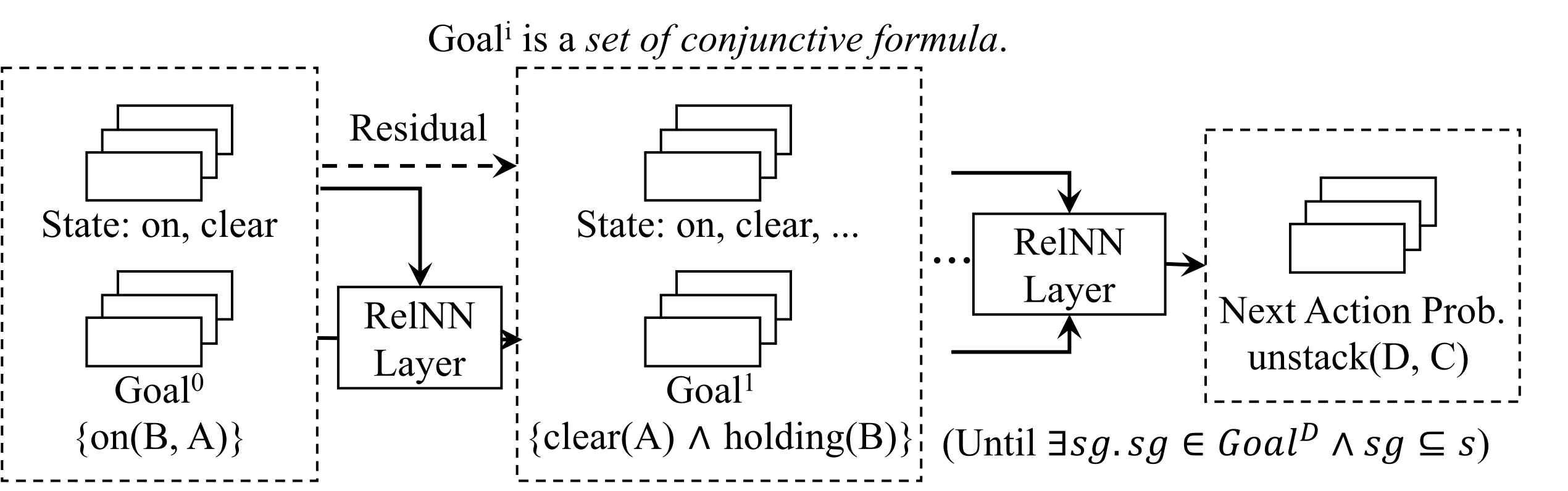
Equations
B.2 Proof of Theorem 4.2: Compilation of S-GRS
The SOS proof uses the forward-width connection to simulate IW(k + 1). The circuit records reachability of small atom tuples and the truth of predicates in a representative terminal state of the associated optimal trajectory. One layer expands by an action. Reapplying the resulting policy follows the selected tuple path; the claimed breadth and depth depend on the preceding width result.
B.3 More Discussion
A recurrent relational layer can perform a number of iterations that grows with instance size. Alternatively, a derived above relation can identify a clear topmost block in one step. Computing that relation is additional work or information supplied by the representation.
The appendix also describes a right-turn/depth-first linearization shortcut for path finding in an acyclic maze. Its topology and representation assumptions matter; it does not establish a fixed-depth optimal policy for arbitrary cyclic navigation problems.
Appendix C Analysis of AI Planning Problems
Table 3 restates the six-domain analysis. The guarantees are for the stated single-atom goal classes; optimal multi-goal planning is generally not serializable by simply achieving each goal once. Super-predicates can address interactions at potentially exponential representation cost.
For satisficing rather than optimal planning, the authors describe simple sequential goal achievement in Logistics, Gripper, Rover, and Elevator. Unbounded-depth domain constructions commonly scale with the number of objects or graph distance, even when relational breadth is constant.
| Problem | Breadth | Regression Width | Depth |
| BlocksWorld | Constant | 1 | Unbounded |
| Logistics | Constant | 0 | Unbounded |
| Gripper | Constant | 0 | Constant |
| Rover | Constant | 0 | Unbounded |
| Elevator | Constant | 0 | Unbounded |
| Sokoban | Unbounded | N/A (not serializable) | Unbounded |
C.1 SOS Width Analysis
The appendix lists domain-specific regression-rule selectors as constructive witnesses for finite SOS width. These rules omit some static type checks and must be read with the domain assumptions.
Finite SOS width for Blocks World.
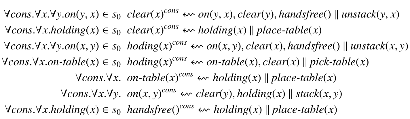
The Blocks World rules choose among unstack, place-table, pick-table, and stack according to current on/holding predicates. Their full seven-line formula array is preserved below. These single-goal constructions underlie the reported SOS width of one.
Equation
Finite SOS width for Logistics.
The Logistics rules regress location goals through unloading, loading, driving, and flying. Static checks such as requiring airport endpoints are omitted in the source. The displayed load/unload arguments use x and y despite quantifying other variable names; the original notation is retained rather than silently repaired.
Equation
Appendix D Experimental Details
Appendix D specifies the three experimental generators, optimizer, compute, and released code.
D.1 Training details
The experiment settings below supplement Table 2’s depth schedules, breadth two, and hidden dimension 64.
Environment setup.
Assembly3 samples three object types and match relations with exactly one compatible A–B–C tuple. BlocksWorld-Clear adds blocks one by one onto a clear block or the table, then selects a target that is initially covered. Logistics grows a directed tree from the starting node and adds a few forward connections before sampling a destination. These structured distributions constrain the generalization claim.
Additional hyperparameters.
All experiments use Adam with learning rate 0.001, β₁ = 0.9, and β₂ = 0.999. Architecture depth varies by task as reported in Table 2.
Compute.
Each experiment uses one NVIDIA Titan RTX GPU on an internal cluster.
Code.
The released goal-regression-width repository contains reproduction code for the experiments.