The paper integrates contraction-based modular control into reinforcement learning. It transforms dynamics into an auxiliary coordinate system, constrains elementary feedback modules, and composes them so that the authors’ stability conditions can be enforced through network Jacobians. Simulated peg tasks illustrate improved robustness and exploration. The guarantees depend on model, transformation, and coupling assumptions; they do not certify arbitrary learned policies or contact environments.
I Introduction
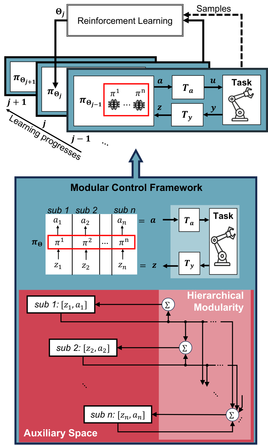
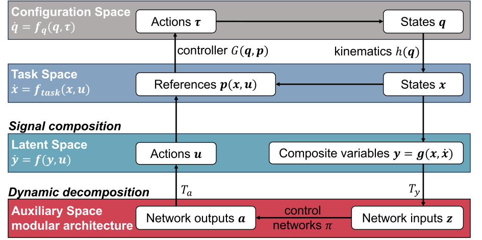
Reward optimization alone can favor policies with unstable behavior for some system parameters. The proposed architecture separates signal composition, which defines the policy’s latent state, from dynamic decomposition, which exposes manageable feedback subsystems. Contraction constraints are imposed on the controller while the usual RL update optimizes rewards. Models or suitable task-space controllers are still needed to construct the transformations.
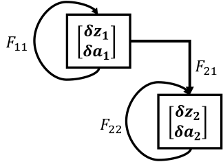
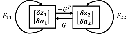
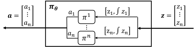
Fig. 1: Modular control framework for RL. The modularity, for example, hierarchical combination of subsystems, is realized in the auxiliary space by coordinate transformation (). Stability can be automatically guaranteed provided each subsystem has stable self-feedbacks, yielding linear constraints on the input gradients of control networks that can be as simple as switching the signs of weights.Fig. 2: Signal flows across different spaces. Signal composition creates the latent space, within which neural control with RL applies to maximizing rewards. Provided that the composition of latent signals is a contracting system, the stability of latent signals implies the stability of physical dynamics. Dynamic decomposition in the auxiliary space further simplifies the stability of latent signals into algebraically solvable ones via modularity.
I-A Technical Contributions.
The central contribution is a coordinate-transformation framework that reduces stability analysis to elementary modules and constrains their input gradients. Additional constructions transfer latent convergence to physical tracking and use task-space controller gains to obtain a usable latent dynamics model.
I-B Related work.
The method connects contraction-based control with modular policy architectures.
Contraction analyzes convergence between trajectories without prescribing an equilibrium. Unlike methods that learn a separate certificate or solve a constrained policy optimization problem, this approach uses stability-preserving interconnections to derive algebraic constraints on the control network. [23], [24], [6].
I-B 2 Modularity
The modularity concerns differential dynamics, beyond simply dividing a network into functions. It is related to motor primitives, synergies, and geometric motion policies, but generalization to underactuated or learned latent modules is proposed rather than demonstrated.
I-C Paper organization
The paper develops decomposition, signal composition, and implementation before presenting simulation experiments and supporting derivations.
II Dynamic decomposition
Coordinate transformations make the closed-loop differential dynamics amenable to modular analysis.
II-A Contraction from auxiliary space to latent space
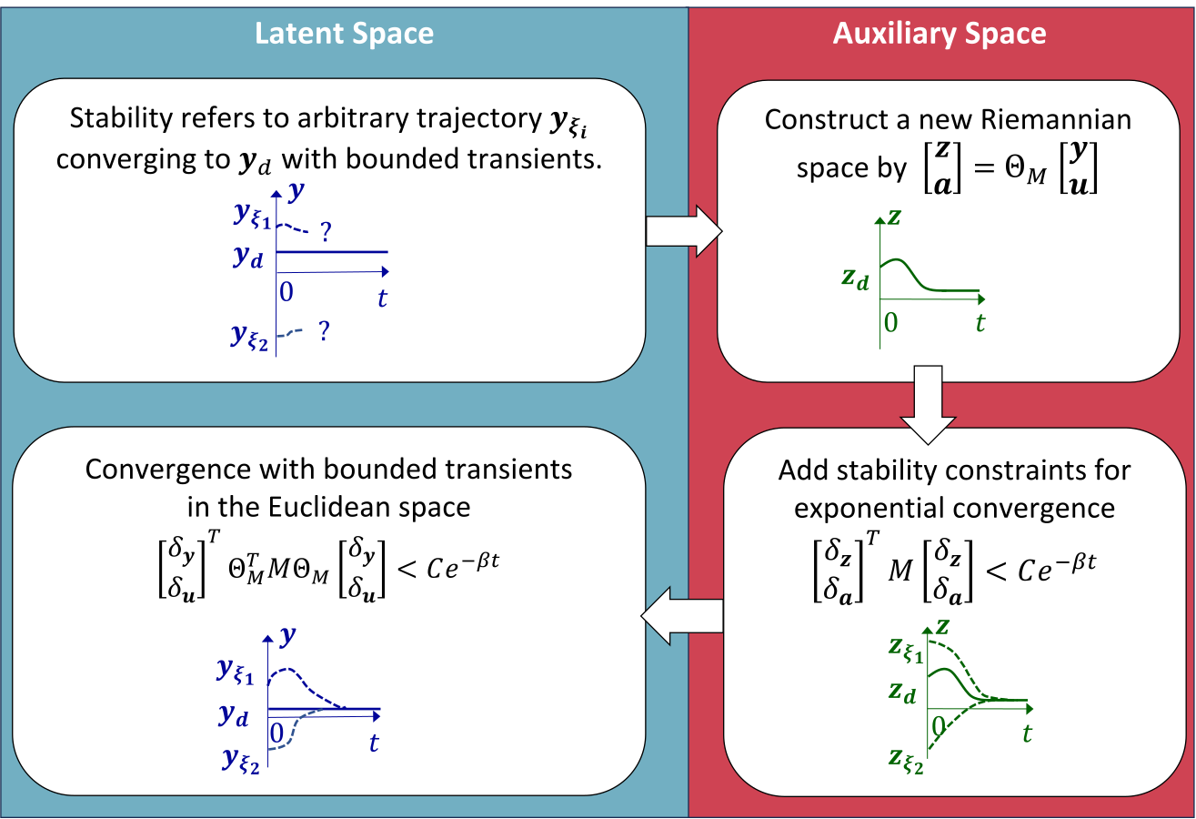
Contraction in auxiliary coordinates transfers to latent dynamics through the induced metric when the transformation has the required positive-definiteness properties. Euclidean trajectories may have bounded transients even when their auxiliary distance contracts.
Fig. 3: By constraining the dynamics in the auxiliary space to converge exponentially, the dynamics in the Euclidean space is converging with bounded transients.
II-B Differential dynamics in the auxiliary space
State and action transformations create auxiliary signals; each policy can use both the current signal and its integral. The block differential model combines plant derivatives and policy Jacobians. The derivation explicitly neglects small changes in the policy input gradient, a restriction relevant to interpreting the resulting conditions.
Equations 1–7
(1)
(2)
(3)
(4)
(5)
(6)
(7)
II-C Modular neural control via dynamic decomposition
Grouping each transformed state with its action yields elementary feedback modules. Triangular couplings permit hierarchical composition, while antisymmetric couplings motivate a feedback alternative. Finding suitable transformations is itself a design problem; the paper develops an explicit hierarchical construction rather than a general existence result.
Equations 8–11
(8)
(9)
(10)
(11)
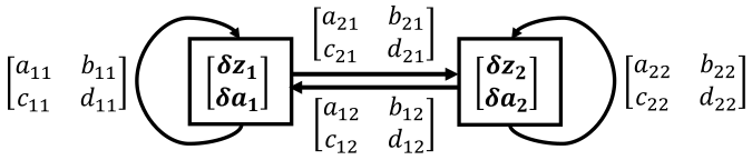
(a)Combination of two subsystems.
(b)Hierarchical combination
(c)Feedback combination
Fig. 4: Combination examples.Equations 12–13
(12)
(13)
Fig. 5: Convergence of hierarchical combinations, where denotes the differential displacements between two arbitrary trajectories at fixed time of the subsystem. When , all possible trajectories of the th subsystem converge to its equilibrium. The subsystems converge recursively following their hierarchies, given stable self-feedback-loops and bounded couplings, as the lowest level with nonzero ’s is always independent.
II-D Explicit solution to the hierarchical-type modularity
The stated hierarchical theorem requires a diagonalizable dynamics Jacobian, suitable uniformly positive-definite transformations, independent per-coordinate policies, bounded couplings, and transformations that stop changing after a finite transient. Eigenvector and QR constructions yield linear inequalities on policy derivatives. These assumptions delimit the stability claim.
Equation 14
(14)
Fig. 6: Independent network for each dimension .
III Signal composition
Stable latent signals alone do not ensure stable physical motion. The signal-composition map must also have stable dynamics. A weighted combination of position and velocity tracking errors provides the worked example; extension to learned latent signals requires additional derivative constraints.
Equation 15
(15)
IV For unknown environments
Unknown external environments can be handled using a task-space controller that shapes end-effector dynamics and admits an added RL command. Its gains then define the latent model. This avoids modeling every environment detail but still requires a robot model and the controller’s tracking assumptions.
V Implementation and limitations
Implementation modifies the policy architecture and controller interface while retaining the underlying RL update.
V-A Implementation
Use composite tracking errors as state, insert coordinate-transform layers, assign an independent network to each transformed coordinate, and enforce the derived Jacobian inequalities. Transformation quantities may be updated each time step.
V-B Further simplification
For already stable nominal dynamics, the constraints reduce to signs of policy derivatives. With nonsaturated tanh activations and suitable weight signs, an MLP can enforce the required monotonicity. This simplification relies on the architecture and baseline stability.
Equations 16–17
(16)
(17)
V-C Limitations
Computational and expressivity costs remain.
Limited control frequency
Repeated eigenvalue and QR decompositions limit achievable control frequency. Designing latent dynamics with a diagonal Jacobian can reduce this cost.
Loss of optimality
Restricting couplings and signal composition may sacrifice control optimality. A separate planner can potentially compensate, but this is not an optimality guarantee.
VI Example 1: Necessity for robustness and generlization
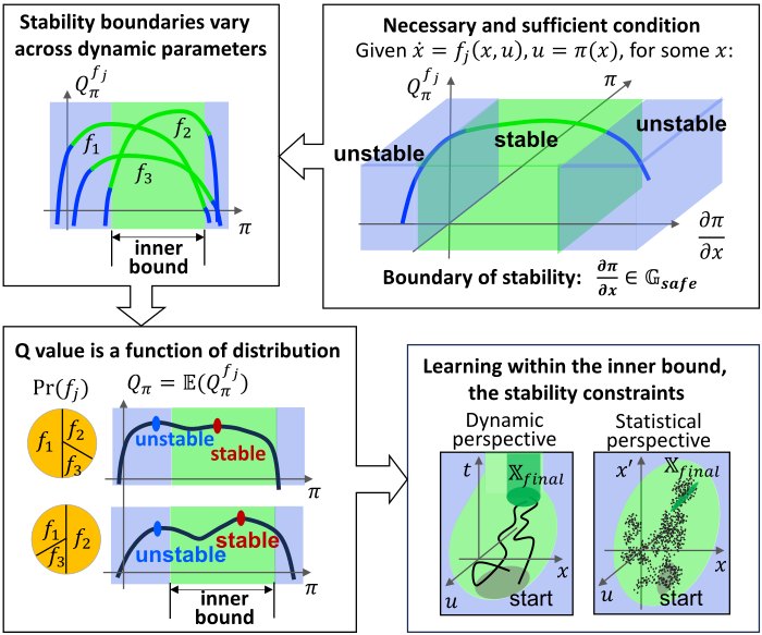
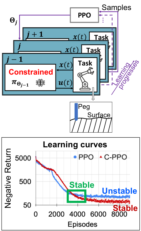
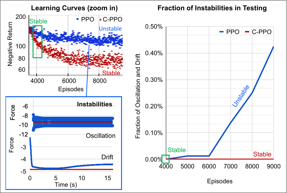
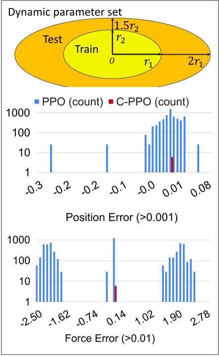
A simulated two-dimensional peg-contact example compares PPO with its constrained version, C-PPO. Unconstrained training increasingly produces oscillation or drift despite good returns; constraints prevent those observed instabilities and improve tests with changed dynamics and surface parameters.
Fig. 7: Intuition. Local optimal policies can contain unstable control because the stability boundaries may not align with the landscape of expected returns.
VII Example 2: Manipulation learning
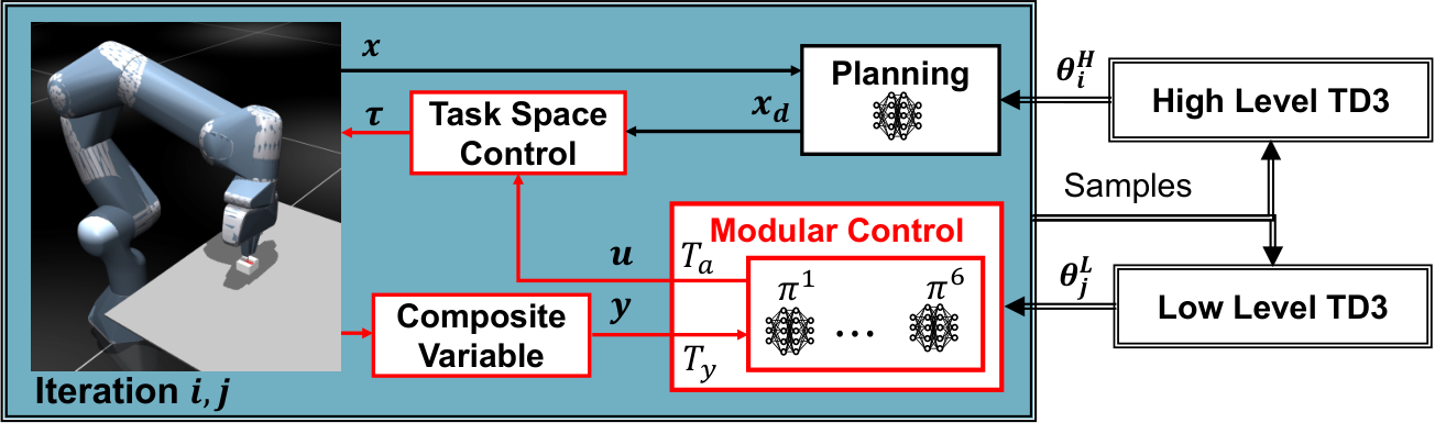
Simulated Franka Panda peg tasks use a slow TD3 planner and a faster constrained TD3 controller. Compared with HIRO, the proposed implementation also changes planning coordinates and removes relabeling, so its advantage cannot be attributed solely to stability constraints. Separate ablations compare unconstrained neural control and fixed non-neural controllers. [17].
Peg Maze compares learning and contact behavior with HIRO.
Task setting.
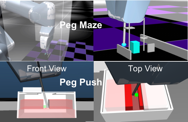
The robot must pass a peg through fixed obstacles under a height-limiting hood to reach a sampled goal.
Experiment
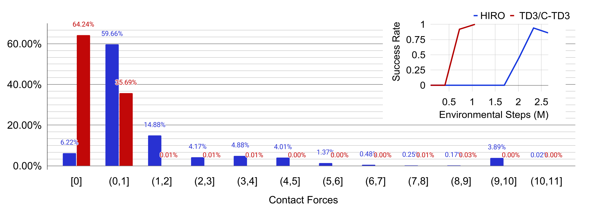
With initial exploration directed toward the maze, the proposed method learns in about one million steps versus two million for HIRO. Contacts below 1 N occur on 99.93% versus 65.88% of sampled steps. The authors attribute benefits to both stable low-level control and easier task-space planning.
VII-B Ablation study: peg-push task
Peg Push tests the role of learned control and contraction constraints.
Task setting
Reaching the hidden target requires opening a sliding lid, entering a narrow slot, and moving an obstacle.
Experiment
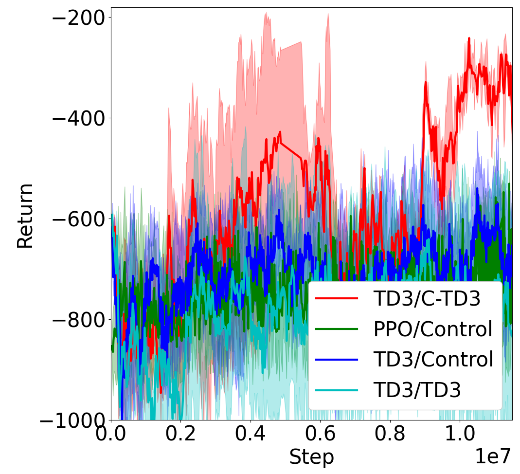
Across five seeds, only TD3/C-TD3 learns the task within the reported 12-million-step budget; two runs converge near three million steps, producing large variation. Fixed controllers learn stable but incomplete routes, while unconstrained hierarchical control passes the goal unstably. Soft-contact penetration is an acknowledged simulator limitation.
VIII Concluding Remarks
Contraction-based modularity offers a structured way to combine control analysis and learned policies. The demonstrated benefits concern simulated manipulation under the specified controller and model assumptions.
IX Appendix
The retained result figures show peg-contact stability tests, parameter-shift robustness, maze contact-force distributions, and peg-push learning curves. The subsequent appendix supplies definitions, proofs, and implementation settings.
(b)Stability: mitigation of oscillation and drift by constraints
(c)Generalization and robustness.
Fig. 8: Necessity for robustness and generalization (more results in [6]). (a) 2D peg-touching task. Both PPO and C-PPO can learn the task with similar return levels and with similar data efficiency. (b) Stability. Starting from the policy at Episode 5000, 8000 trajectories are tested every 1k episodes. In PPO, the amount of oscillation and drift is increasing as learning progresses, which implies overfitting, while in C-PPO, the fraction remains zero. (c) Generalization and robustness. The policies at Episode 5000 are tested for 8000 trajectories, with new task parameters with differences in (), in and in () compared to the training set. The nominal model from the training set is used in C-PPO. The histogram of tracking errors shows dramatic improvements in generalization in C-PPO.
(a)Hierarchical RL with stable modular neural control in the low level (TD3/C-TD3).
(b)Peg maze and peg push.
(c)Peg maze: Contact force distributions and the success rates.
(d)Peg push: Learning curves.
Fig. 9: Effectiveness in manipulation learning (trajectory examples in https://www.youtube.com/watch?v=nFLHwVfPIJw for peg maze and https://www.youtube.com/watch?v=RpGzpZPifUw for peg push.) (a) Hierarchical RL framework of TD3/C-TD3. (b) Peg maze and peg push tasks. Peg maze (top) is a goal reaching task with fixed obstacles both near the goal (randomly sampled in the green zone) and near the robot arm (the transparent hood). Peg push (bottom) is a goal reaching task that requires opening a sliding lid box, inserting into a deep slot, and pushing away the green obstacle to reach the small red spot underneath. (c) Peg maze results: TD3/C-TD3 vs. HIRO (the state-of-the-art data-efficient hierarchical RL). Both TD3/C-TD3 and HIRO can quickly learn the task (1M and 2M steps). The contact force distribution are estimated from policies (success rates on top right) at 10k, 200k, 400k, 600k, 800k, and 1M steps for TD3/C-TD3, and at 10k, 500k, 1M, 1.5M, 2M, and 2.3M steps for HIRO. The distribution shows improvements in safe exploration that in TD3/C-TD3, are with less than 1 N, and with HIRO. (d) Peg push results: TD3/C-TD3 vs. RL with non-neural controllers (PPO/Control, TD3/Control) vs. TD3/TD3 without stability constraints. Only TD3/C-TD3 successfully learn the task within 12 M steps, with 2 trials learned the task around 3 M steps causing the large variation. TD3/control and PPO/control can learn stable trajectories but haven’t figured out the entire path to the goal. Without stability constraints, TD3/TD3 learns unstable trajectories passing by the goal.
Acknowledgments
Support came from the RIE2020 industry collaboration initiative and the HP–NTU Digital Manufacturing Corporate Lab.
X Appendix
The technical appendix makes the stability assumptions and experimental settings explicit.
X-A Incremental exponential stability
Incremental exponential stability bounds the distance between any two trajectories by an exponentially decaying multiple of their initial separation.
Equation 18
(18)
X-B Stability theorem for smooth coordinate transformation
The coordinate-transformation theorem requires a uniformly negative symmetric part of the transformed differential dynamics, with margin for time-varying transformation terms. It establishes the paper’s regional convergence claim under these stated conditions.
Equations 19–21
(19)
(20)
(21)
Differential dynamics in the auxiliary space
The transformed differential matrix includes plant derivatives, policy input gradients, and the derivative of the state transformation.
Equations 22–24
(22)
(23)
(24)
Sufficient condition that makes the squared distance between trajectories exponentially converge in the auxiliary space
Differentiating squared auxiliary distance gives an exponential bound when the symmetric part of the differential matrix is uniformly negative.
Equations 25–26
(25)
(26)
Distance between two arbitrary trajectories
A lower bound on the induced metric relates auxiliary path length to separation in the original coordinates, yielding a transient multiplier and exponential rate.
Equation 27
(27)
Boundary for the constant part in F
The time-varying matrix contribution is bounded separately; the nominal contraction margin must dominate its largest symmetric-part eigenvalue.
Equation 28
(28)
X-C Proof of the theorem for the hierarchical combination.
The hierarchical construction simplifies these conditions using triangular interconnections.
X-C 1 Assumption that the term involving F 2 in Eq. ( 21 ) can be seen as bounded temporary disturbances
The proof assumes transformation changes end after a finite time and trajectory separation remains bounded before then. Arbitrarily persistent transformation variation is outside this simplification.
X-C 2 Differential dynamics in the auxiliary space
After the transient, the reduced differential system applies exactly. Before it, the bounded separation is absorbed into the exponential bound’s prefactor.
Equation 29
(29)
X-C 3 Diagonal Λ via T y
A coordinate basis diagonalizes the latent-state Jacobian when the required eigendecomposition exists.
Equation 30
(30)
X-C 4 Upper triangular R via T a
A QR factorization and reversal permutation construct an action transformation with upper-triangular input coupling.
Equations 31–33
(31)
(32)
(33)
X-C 5 Hierarchical combination of subsystems
Independent coordinate policies preserve this triangular structure. Regrouping state and action displacements exposes a hierarchy of two-dimensional modules.
Equations 34–39
(34)
(35)
(36)
(37)
(38)
(39)
X-C 6 Linear constraints from the preservation of contraction
The paper derives derivative inequalities from each module’s characteristic polynomial and uses its hierarchical contraction argument to obtain the stated stability condition. This is a sufficient-design construction under the earlier assumptions, not an unrestricted test for nonlinear feedback stability.
Equations 40–43
(40)
(41)
(42)
(43)
X-D Integration of composite variables and task space controllers for unknown environments
Task-space control supplies a more tractable latent model when the external environment is not explicitly known.
X-D 1 Reference 𝐩 ( 𝐱 , 𝐮 ) in task space control
Rigid-body compensation and a Jacobian-based controller shape end-effector errors into a second-order system with an added learned input.
Equations 44–49
(44)
(45)
(46)
(47)
(48)
(49)
X-D 2 Composite variables for a given 𝐩 ( 𝐱 , 𝐮 )
Combining position and velocity errors yields first-order latent dynamics. The displayed gain solution requires a nonnegative discriminant in each controlled dimension; a zero position gain instead permits a velocity-error signal.
Equations 50–54
(50)
(51)
(52)
(53)
(54)
X-D 3 Stability constraints
Positive diagonal latent coefficients allow identity transformations and reduce the proposed inequalities to positive policy input gradients.
Equation 55
(55)
X-E Robustness
Two robustness analyses bound disturbances and model mismatch.
X-E 1 Robustness to unknown deterministic perturbation
For a contracting system with bounded metric and bounded disturbances, trajectory error approaches a ball whose size grows with disturbance magnitude and shrinks with contraction rate. Applying this result to the augmented state also requires bounded transformations and network gradients.
Equations 56–61
(56)
(57)
(58)
(59)
(60)
(61)
X-E 2 Robustness to model errors
Model errors preserve the argument when the real transformed symmetric dynamics remain dominated by the nominal stability bound. This is a conditional robustness criterion, not tolerance of arbitrary model error.
The PPO example uses first-order peg dynamics and a random sinusoidal surface with sampled stiffness and goals.
Equations 64–65
(64)
(65)
Computation of T y , T a , Λ i i , and R i i
Contact dynamics are expressed in horizontal position and force. Approximate plant derivatives determine the transformations and constraint coefficients at each step.
Three-layer tanh networks use positive weights and a conditional output sign flip to obtain the required derivative signs. The retained tables provide maze hyperparameters, peg-push geometry, controller gains, and TD3 settings.
Maze success requires position error below 5 mm. Task-space and joint-space baselines use separately tuned controller and action ranges; these implementation differences matter when interpreting the comparison.
X-H Peg-Push Example
Peg Push uses MuJoCo soft-contact settings, 50 Hz control, a 2.5 Hz planner, and 20-second trajectories. Planner increments are bounded by 5 mm and 0.5 radians; the appendix retains geometry, rewards, gains, and learning settings.
32 references
[1]
R. Cheng, A. Verma, G. Orosz, S. Chaudhuri, Y. Yue, and J. Burdick, “Control
regularization for reduced variance reinforcement learning,” in
International Conference on Machine Learning. PMLR, 2019, pp. 1141–1150.
[2]
F. Berkenkamp, M. Turchetta, A. P. Schoellig, and A. Krause, “Safe model-based
reinforcement learning with stability guarantees,” arXiv preprint
arXiv:1705.08551, 2017.
[3]
S. Singh, V. Sindhwani, J.-J. E. Slotine, and M. Pavone, “Learning
stabilizable dynamical systems via control contraction metrics,” in
International Workshop on the Algorithmic Foundations of
Robotics. Springer, 2018, pp.
179–195.
[4]
A. Mandlekar, Y. Zhu, A. Garg, L. Fei-Fei, and S. Savarese, “Adversarially
robust policy learning: Active construction of physically-plausible
perturbations,” in 2017 IEEE/RSJ International Conference on
Intelligent Robots and Systems (IROS). IEEE, 2017, pp. 3932–3939.
[7]
C. Dawson, S. Gao, and C. Fan, “Safe control with learned certificates: A
survey of neural lyapunov, barrier, and contraction methods,” arXiv
preprint arXiv:2202.11762, 2022.
[8]
N. Boffi, S. Tu, N. Matni, J.-J. Slotine, and V. Sindhwani, “Learning
stability certificates from data,” in Conference on Robot
Learning. PMLR, 2021, pp. 1341–1350.
[9]
Z. Qin, K. Zhang, Y. Chen, J. Chen, and C. Fan, “Learning safe multi-agent
control with decentralized neural barrier certificates,” arXiv
preprint arXiv:2101.05436, 2021.
[10]
Y. Luo and T. Ma, “Learning barrier certificates: Towards safe reinforcement
learning with zero training-time violations,” Advances in Neural
Information Processing Systems, vol. 34, pp. 25 621–25 632, 2021.
[11]
H. Ma, C. Liu, S. E. Li, S. Zheng, and J. Chen, “Joint synthesis of safety
certificate and safe control policy using constrained reinforcement
learning,” in Learning for Dynamics and Control Conference. PMLR, 2022, pp. 97–109.
[12]
S. Reed, K. Zolna, E. Parisotto, S. G. Colmenarejo, A. Novikov, G. Barth-Maron,
M. Gimenez, Y. Sulsky, J. Kay, J. T. Springenberg et al., “A
generalist agent,” arXiv preprint arXiv:2205.06175, 2022.
[13]
J.-J. Slotine and W. Lohmiller, “Modularity, evolution, and the binding
problem: a view from stability theory,” Neural networks, vol. 14,
no. 2, pp. 137–145, 2001.
[14]
J.-J. E. Slotine, “Modular stability tools for distributed computation and
control,” International Journal of Adaptive Control and Signal
Processing, vol. 17, no. 6, pp. 397–416, 2003.
[15]
J. Nakanishi, R. Cory, M. Mistry, J. Peters, and S. Schaal, “Operational space
control: A theoretical and empirical comparison,” The International
Journal of Robotics Research, vol. 27, no. 6, pp. 737–757, 2008.
[16]
S. Fujimoto, H. Hoof, and D. Meger, “Addressing function approximation error
in actor-critic methods,” in International conference on machine
learning. PMLR, 2018, pp. 1587–1596.
[17]
O. Nachum, S. S. Gu, H. Lee, and S. Levine, “Data-efficient hierarchical
reinforcement learning,” Advances in neural information processing
systems, vol. 31, 2018.
[18]
E. M. Aylward, P. A. Parrilo, and J.-J. E. Slotine, “Stability and robustness
analysis of nonlinear systems via contraction metrics and sos programming,”
Automatica, vol. 44, no. 8, pp. 2163–2170, 2008.
[19]
H. Tsukamoto, S.-J. Chung, and J.-J. E. Slotine, “Neural stochastic
contraction metrics for learning-based control and estimation,” IEEE
Control Systems Letters, vol. 5, no. 5, pp. 1825–1830, 2020.
[21]
H. Tsukamoto and S.-J. Chung, “Learning-based robust motion planning with
guaranteed stability: A contraction theory approach,” IEEE Robotics
and Automation Letters, vol. 6, no. 4, pp. 6164–6171, 2021.
[22]
S. Singh, S. M. Richards, V. Sindhwani, J.-J. E. Slotine, and M. Pavone,
“Learning stabilizable nonlinear dynamics with contraction-based
regularization,” The International Journal of Robotics Research,
vol. 40, no. 10-11, pp. 1123–1150, 2021.
[23]
S. Lale, Y. Shi, G. Qu, K. Azizzadenesheli, A. Wierman, and A. Anandkumar,
“Kcrl: Krasovskii-constrained reinforcement learning with guaranteed
stability in nonlinear dynamical systems,” arXiv preprint
arXiv:2206.01704, 2022.
[25]
M. Jin and J. Lavaei, “Stability-certified reinforcement learning: A
control-theoretic perspective,” IEEE Access, vol. 8, pp.
229 086–229 100, 2020.
[26]
K. A. Thoroughman and R. Shadmehr, “Learning of action through adaptive
combination of motor primitives,” Nature, vol. 407, no. 6805, pp.
742–747, 2000.
[27]
M. Santello, M. Bianchi, M. Gabiccini, E. Ricciardi, G. Salvietti,
D. Prattichizzo, M. Ernst, A. Moscatelli, H. Jörntell, A. M. Kappers
et al., “Hand synergies: Integration of robotics and neuroscience for
understanding the control of biological and artificial hands,” Physics
of life reviews, vol. 17, pp. 1–23, 2016.
[30]
H. Tsukamoto, S.-J. Chung, and J.-J. E. Slotine, “Contraction theory for
nonlinear stability analysis and learning-based control: A tutorial
overview,” Annual Reviews in Control, 2021.
[32]
M. Parmar, M. Halm, and M. Posa, “Fundamental challenges in deep learning for
stiff contact dynamics,” in 2021 IEEE/RSJ International Conference on
Intelligent Robots and Systems (IROS). IEEE, 2021, pp. 5181–5188.