Dynamic movement primitives (DMPs) parameterize motion trajectories; elementary dynamic actions (EDAs) combine submovements, oscillations, and mechanical impedances. This edition follows the requested 2023 preprint, which compares them through eight simulated control examples. The later journal publication is linked above. The comparison emphasizes trajectory reproduction, contact behavior, singularities, and composition rather than ranking one method universally better.
1 Introduction
Both approaches build complex movement from reusable primitives, but at different levels. DMPs learn a forcing function within an attractor-based trajectory generator. EDAs separate a virtual movement from the mechanical response connecting it to the robot. The paper compares particular torque-control implementations and suggests combining their strengths; its findings should not be read as restrictions on every possible DMP controller.
2 Theory
The theory begins with one degree of freedom (DOF) before extending the constructions to robot joints and end-effector motion.
2.1 Dynamic Movement Primitives
A DMP consists of a phase-generating canonical system, a learned nonlinear forcing term, and a transformation system producing motion. Discrete and rhythmic variants use different phase and basis functions.
2.1.1 Canonical System
Discrete phase decays exponentially toward zero; rhythmic phase advances around a cycle. A time constant controls movement speed and duration.
Equation 1
(1)
2.1.2 Nonlinear Forcing Term
Weighted Gaussian bases shape discrete movements, while periodic von Mises bases shape rhythmic ones. Start/goal displacement or oscillation amplitude scales the forcing term.
Equations 2–3
(2)
(3)
2.1.3 Transformation System
A second-order transformation system resembles a damped spring driven by the learned force. With a vanishing discrete forcing term and suitable positive gains, it converges toward the goal. Phase supplies a reusable progression variable rather than an explicit time-indexed trajectory.
Equation 4
(4)
2.1.4 Imitation Learning
Demonstrated positions, velocities, and accelerations determine a target forcing function. Locally weighted or least-squares regression fits its basis weights. The resulting motion can be rescaled in time and space, and multiple joints share one phase variable. Reproduction accuracy depends on the representation, data, and subsequent robot controller; fitting a forcing function does not itself guarantee perfect physical tracking.
Equations 5
(5)
2.2 Elementary Dynamic Actions
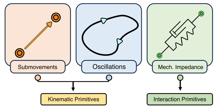
EDAs use three primitive types: finite submovements, periodic oscillations, and mechanical impedances that govern interaction.
Fig. 1: The three primitives of Elementary Dynamic Actions (EDAs). Submovements and oscillations correspond to kinematic primitives and mechanical impedances manage physical interaction.
2.2.1 Submovements
A submovement is a smooth finite-duration displacement with a single-peaked velocity profile. Its amplitude, duration, timing, and shape parameterize a discrete motion.
Equation
2.2.2 Oscillations
An oscillation supplies a smooth periodic virtual trajectory. More general almost-periodic motions are possible, but the examples use ordinary periodic functions.
Equation
2.2.3 Mechanical Impedances
Mechanical impedance maps displacement from a virtual trajectory to interaction force, including stiffness, damping, and more general dynamics. Compatible impedance operators can be superimposed, with Jacobian-transpose maps converting task-space forces to joint torques. Stability and passivity depend on the operators and interconnection assumptions.
Equations 6–7
(6)
(7)
2.2.4 Norton Equivalent Network Model
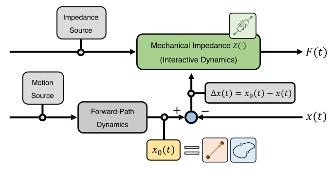
The Norton-equivalent view separates the virtual trajectory from the impedance connecting it to the actual robot motion. Neither position nor force is directly prescribed: both arise from interaction with the environment. Submovements and oscillations can be added at the trajectory level, while impedance components can be combined at the force level.
Fig. 2: The three Elementary Dynamic Actions (EDAs) combined using a Norton equivalent network model. The virtual trajectory (yellow box) consists of submovements (orange box) and/or oscillations (blue box), and mechanical impedance (green box) regulates the interactive dynamics.
3 Comparison of the Two Approaches
Eight MuJoCo examples compare reaching, contact, avoidance, rhythmic motion, combined motions, sequencing, and redundancy. The models assume ideal torque actuation and gravity compensation; end-effector orientation is omitted. These are explanatory simulations, not a hardware benchmark or statistical evaluation.
Equation 8
(8)
3.1 The Existence of an Inverse Dynamics Model
The implementations differ in how a generated motion becomes a torque command.
3.1.1 Dynamic Movement Primitives
The chosen DMP implementation converts desired kinematics to feedforward torque through inverse dynamics, adding feedback for disturbance rejection. Task-space trajectories additionally require inverse kinematics or related feedback mappings. Exact tracking claims assume an accurate model and favorable operating conditions.
3.1.2 Elementary Dynamic Actions
The EDA implementation maps measured displacement and velocity through joint/task impedances to torque. It needs state measurements and forward kinematics but not a full inverse dynamics model for these examples. More advanced impedance shaping may require additional model knowledge.
Equation
3.2 A Goal-directed Discrete Movement in Joint-space
The first example reaches a target joint configuration along a specified motion.
3.2.1 Dynamic Movement Primitives
Each joint has a DMP transformation system synchronized by a common phase. A learned force reproduces the desired trajectory, whose position, velocity, and acceleration feed the inverse dynamics controller.
Equation 9
(9)
3.2.2 Elementary Dynamic Actions
Joint-space stiffness and damping connect the robot to a finite virtual submovement ending at the goal. Under the stated conditions, the configuration converges to that goal even when it does not track the virtual trajectory exactly.
Equation 10
(10)
3.2.3 Simulation Example
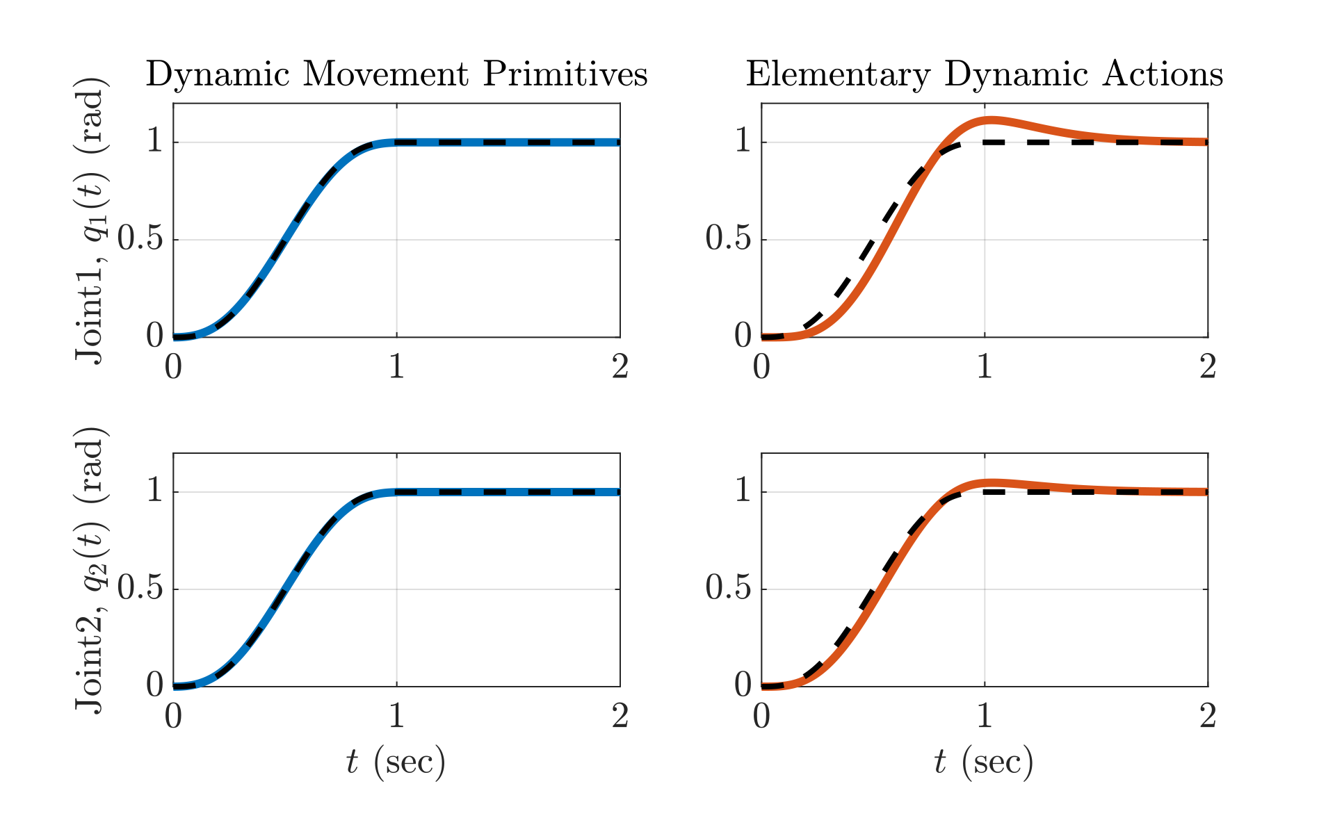
A two-link planar arm follows minimum-jerk joint movements. The ideal-model DMP controller closely tracks the specified motion; the impedance controller exhibits transient tracking error but reaches the target without inverse dynamics.
Equation 11
(11)
Fig. 3: A goal-directed discrete movement in joint-space for Dynamic Movement Primitives (DMPs, blue) and Elementary Dynamic Actions (EDAs, orange) (Section 3.2.3). The black dotted line is a minimum-jerk trajectory (Equation (11)). Goal location: rad. Parameters of minimum-jerk trajectory: rad, s. Parameters of DMPs: , , , , , , for , for , . Parameters of EDAs: Nm/rad, Nms/rad, where is an identity matrix. For DMP, perfect tracking was achieved. For EDA, a non-negligible tracking error was observed.
3.3 A Goal-directed Discrete Movement in Task-space
The next example reaches in Cartesian task space, including a target at a fully extended singular configuration.
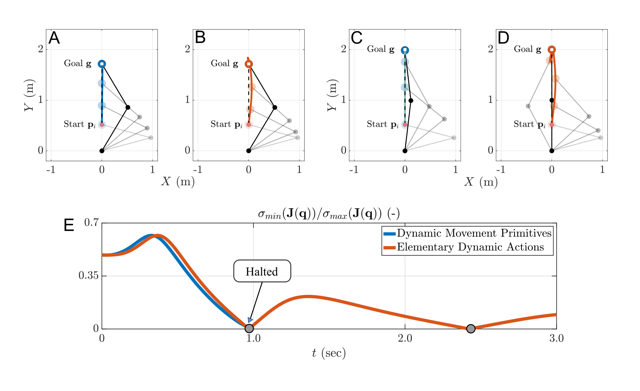
Fig. 4: A goal-directed discrete movement in task-space for (A, C, E) Dynamic Movement Primitives (DMPs, blue) and (B, D, E) Elementary Dynamic Actions (EDAs, orange) (Section 3.3.3). (A, B, C, D) Goal-directed discrete movements in a direction along the positive -axis direction, but (C, D) reached kinematic singularity. The black dotted line is a minimum-jerk trajectory (Equation (14)).
(E) Time vs. of both robots for (C, D), where is a singular value of the matrix. For DMPs, the MuJoCo simulation halted near 0.99s.
Parameters of a minimum-jerk trajectory: (A, B) m, m, s (C, D) m, m, s, where is the initial end-effector position.
Parameters of DMPs are identical to those in Figure 3.
Parameters of EDAs: N/m, Ns/m. For DMP, perfect tracking was achieved when the motion was not near a kinematic singularity. However for (C) when the goal was at a kinematic singularty, the approach failed to achieve the task. For EDA, a non-negligible tracking error existed, but goal-directed discrete movements were achieved for both (A) and (C). The approach based on EDA was not only stable near and at a kinematic singularity but even passed through it (E, near and , depicted as grey circle markers).
.
3.3.1 Dynamic Movement Primitives
DMP-generated Cartesian kinematics are mapped to joints using the Jacobian inverse before inverse dynamics is applied. The simple inverse requires a square, nonsingular Jacobian; redundancy and singularities need additional handling.
Equations 12
(12)
3.3.2 Elementary Dynamic Actions
Task-space stiffness and damping produce a Cartesian force mapped to torque by the Jacobian transpose. This avoids Jacobian inversion, so the command remains defined at a singularity. Goal convergence still relies on the controller’s stated assumptions.
Equation 13
(13)
3.3.3 Simulation Example
Both controllers reach ordinary targets, but the unregularized DMP inverse becomes numerically unstable near full extension. The EDA controller crosses the singularity without numerical failure, though it oscillates because task-space damping cannot dissipate all joint motion there. Joint damping can reduce this oscillation; damped inverse methods and feedback can address the DMP implementation’s difficulty.
Equation 14
(14)
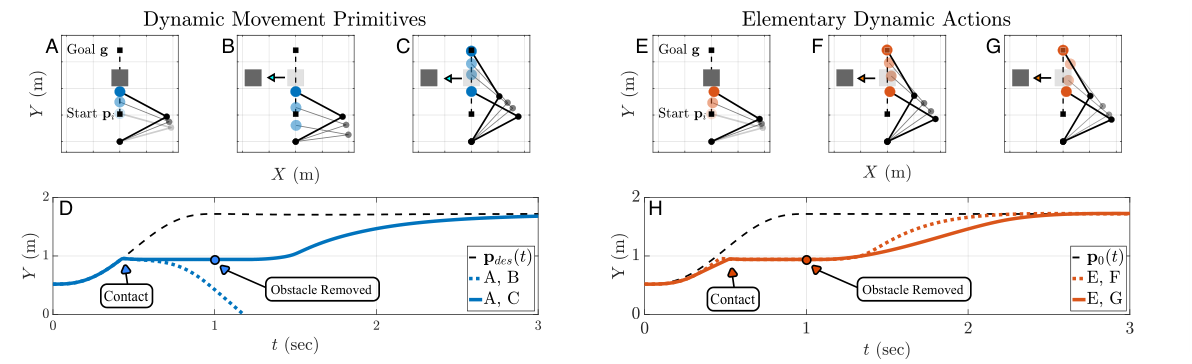
Fig. 5: A goal-directed discrete movement with unexpected physical contact for (A, B, C, D) Dynamic Movement Primitives (DMPs, blue) and (E, F, G, H) Elementary Dynamic Actions (EDAs, orange) (Section 3.4.3). For DMP: (A) Moment of contact. (AB) DMP without PD controller (AC) DMP with PD controller.
(D) Time vs. -coordinate of the end-effector for AB (dotted line) and AC (filled line). For EDA: (E) Moment of contact. (EF) EDA without impedance modulation (EG) EDA with impedance modulation.
(H) Time vs. -coordinate of the end-effector for EF (dotted line) and EG (filled line). With impedance modulation of EG, a slower movement than EF was achieved. (D, H) The black dotted lines are a minimum-jerk trajectory (Equation (14)).
Parameters of the minimum-jerk trajectory, DMPs and EDAs are identical to those in Figure 4. Parameters of the PD controller of DMPs (Equation (15)): Nm/rad, Nms/rad. Smaller gain values than Figure 3 were chosen to achieve a relatively low-gain PD controller as recommended by (Schaal et al., 2007; Pastor et al., 2013).
Parameters of EDAs: J.
3.4 Tasks with Unexpected Physical Contact
An obstacle unexpectedly interrupts a reaching movement and is later removed.
3.4.1 Dynamic Movement Primitives
A low-gain proportional–derivative (PD) feedback torque is added to the DMP feedforward command. This helps recover after contact while reusing the learned trajectory. It is equivalent to one simple joint impedance only under ideal torque actuation.
Equation 15
(15)
3.4.2 Elementary Dynamic Actions
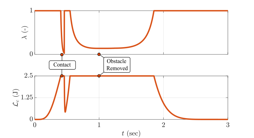
The EDA controller changes stiffness and damping through an energy-dependent scaling factor. The example bounds the combined kinetic and elastic energy under its specified conditions; if kinetic energy already exceeds the threshold, scaling is clipped to prevent negative stiffness. This simplified demonstration is not a general contact-safety certification.
Equations 16
(16)
3.4.3 Simulation Example
The feedforward-only DMP controller rebounds and misses the goal; adding feedback permits recovery. Both EDA variants eventually reach the goal, but energy modulation reduces the large acceleration released when the obstacle is removed.
Fig. 6: Simulation results using Elementary Dynamic Actions (EDAs) with impedance modulation via energy regulation (Equation (16)) (Figure 5) (Section 3.4.3). (Top) Time vs. of the controller. After the first contact, a sudden change in occurred.
(Bottom) Time vs. of the controller. Since the zero-force trajectory continued during contact, the decrease of limited to a maximal value of J.
As expected, did not exceed J.
3.5 Obstacle Avoidance
A known stationary obstacle lies along the nominal reaching path.
3.5.1 Dynamic Movement Primitives
A coupling term steers the DMP acceleration away from the obstacle while retaining the learned forcing weights. This illustrates online trajectory modulation rather than refitting a demonstration.
Equations 17
(17)
3.5.2 Elementary Dynamic Actions
A repulsive impedance is added to the goal-attracting task-space impedance. The resulting force changes the actual motion without explicitly constructing a new collision-free path.
Equation 18
(18)
3.5.3 Simulation Example
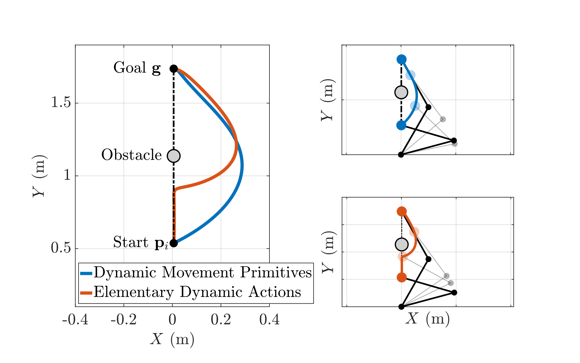
Both implementations avoid the illustrated obstacle. The EDA example needs a manually chosen 2 cm lateral offset to select a useful direction; without it the arm can stall or collide with a link. The result therefore does not establish complete obstacle avoidance from arbitrary starts.
Fig. 7: A goal-directed discrete movement with obstacle avoidance for Dynamic Movement Primitives (DMPs, blue) and Elementary Dynamic Actions (EDAs, orange) (Section 3.5.3). (Left) Trajectory of the end-effector position. Initial end-effector position and goal location are depicted as black circle markers. (Right) Time-lapse of the movement for DMP (Top, blue) and EDA (Bottom, orange). Dotted lines are a minimum-jerk trajectory. Obstacle location m. Parameters of DMPs: , (Equation (17)). Parameters of EDAs: N/m5, (Equation (18)). Other parameters are identical to those in Figure 4.
3.6 Rhythmic Movement
Rhythmic examples use sinusoidal joint motion and a circular end-effector path.
3.6.1 Dynamic Movement Primitives
Periodic DMP phase and forcing functions generate the reference kinematics, followed by the same joint/task mapping and inverse dynamics used earlier.
3.6.2 Elementary Dynamic Actions
A periodic virtual trajectory drives the existing joint-space or task-space impedance controller.
3.6.3 Simulation Example
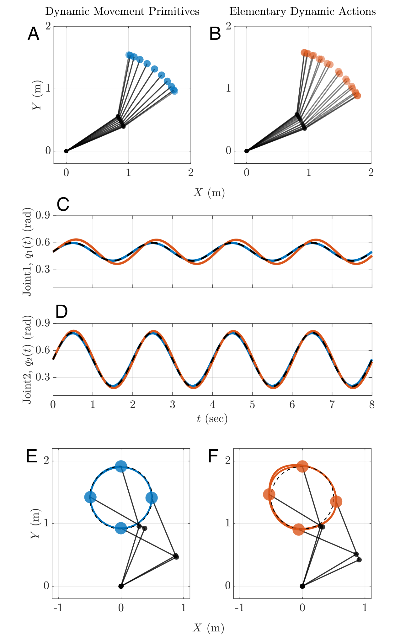
Both methods generate periodic motion. The ideal-model DMP controller reproduces the reference closely, while EDAs exhibit tracking error but avoid inverse dynamics and explicit inverse kinematics in these examples.
Equations 19–20
(19)
(20)
Fig. 8: Rhythmic movements in (A, B, C, D) joint-space and (E, F) task-space for Dynamic Movement Primitives (DMPs, blue) and Elementary Dynamic Actions (EDAs, orange) (Section 3.6.3). (A, B) Rhythmic movement in joint-space and its (C, D) joint trajectories. (C, D) The black dashed lines which are perfectly overlapped with DMPs (blue lines) represent a sinusoidal trajectory with parameters: rad, rad, rad/s (Equation (19)). Parameters of rhythmic DMP: , , , , , , , for . Parameters of EDA are identical to those in Figure 3. (E, F) Rhythmic movement in task-space. The black dashed lines represent a circular trajectory with parameters: m, m, rad/s (Equation (20)).
Parameters of EDAs: N/m, Ns/m. Higher stiffness and damping values than Figure 4 were chosen to reduce the tracking error.
Parameters of rhythmic DMP are identical to those in (A, B). Consistent with Figure 3 and Figure 4, for DMP, perfect tracking was achieved while for EDA, a non-negligible tracking error existed.
3.7 Combination of Discrete and Rhythmic Movements
The next examples shift the center of an ongoing rhythmic movement.
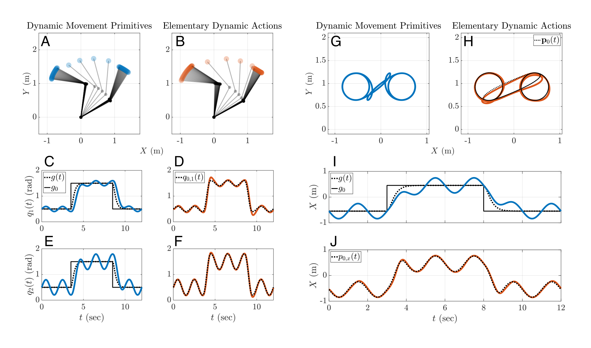
Fig. 9: A combination of discrete and rhythmic movements in (A-F) joint-space and (G-J) task-space for Dynamic Movement Primitives (DMPs, blue) and Elementary Dynamic Actions (EDAs, orange) (Section 3.7.3). (C, E, I) Black filled lines represent the discrete change of of DMP. Black dotted lines represent , which follows a response of a (critically damped) second-order linear system. (D, F, J) Black dotted lines represent and for joint-space and task-space, respectively. (A-F) Parameters of the discrete and rhythmic movements in joint-space: rad/s, rad, rad, rad. (G-J) Parameters of the discrete and rhythmic movements in task-space: rad/s, m, m, m.
In joint-space (respectively task-space), multiple discrete movements in opposite directions are generated by switching the values of (respectively ) and (respectively ), with time offset , where is the number of discrete movements.
Parameters of discrete DMPs in both joint-space and task-space: , , . Other parameters of DMP are identical to those in Figure 8. Parameters of EDA are identical to those in Figure 8. For EDA, given a single impedance operator, discrete and rhythmic movements can be directly combined at the level of the virtual trajectory.
3.7.1 Dynamic Movement Primitives
A discrete system generates a smoothly changing goal for the rhythmic DMP. This couples the two types rather than adding their learned forcing weights directly.
Equation
3.7.2 Elementary Dynamic Actions
A finite submovement is directly added to an oscillation to form the virtual trajectory, leaving the impedance controller unchanged.
Equation
3.7.3 Simulation Example
Both constructions produce combined discrete and rhythmic motion. The selected DMP goal change follows a second-order system, while the EDA construction allows a freely chosen submovement profile. This illustrates the simplicity of virtual-trajectory superposition for the chosen formulations.
Equations
3.8 Sequence of Discrete Movements
A newly appearing target interrupts a discrete reach and requires a smooth redirection.
3.8.1 Dynamic Movement Primitives
Low-pass filtering the DMP goal avoids acceleration discontinuities. In the construction studied here, the initial learned motion is followed by a goal-change response governed by a third-order linear system.
Equations 21
(21)
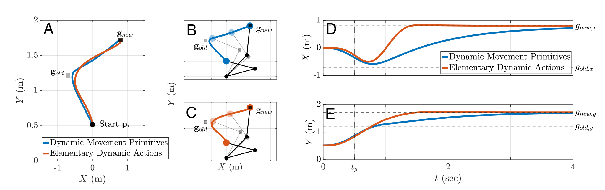
Fig. 10: A sequence of discrete movements for (A, B, D, E) Dynamic Movement Primitives (DMPs, blue) and (A, C, D, E) Elementary Dynamic Actions (EDAs, orange) (Section 3.8.3). (A) Trajectory of the end-effector position. (B, C) Time-lapse of the movement of the 2-DOF robot model. (D, E) Time vs. - and -coordinates of the end-effector trajectory. (A, B, C) The first movement headed toward (square grey marker), but at time (D, E), the target switched location to (square black marker) which necessitated a second movement. Parameters of DMPs (for the first discrete movement): , . Other parameters are identical to those in Figure 4. Parameters of EDAs: s, s, s. m, m, m. Other parameters are identical to those in Figure 4. (D, E) For the new goal location , EDA achieved faster convergence than DMP. For DMP the second movement followed a response of a third-order linear system. On the other hand for EDA, the basis function of the second movement can be freely chosen. Hence, faster convergence to was achieved for EDA.
3.8.2 Elementary Dynamic Actions
A second submovement is superimposed on the first virtual trajectory, with amplitude measured from the previous goal to the new goal. Each submovement may use its own smooth basis.
Equation
3.8.3 Simulation Example
Both controllers converge to the newly supplied goal. The selected EDA profiles reach it faster in this example, and the first submovement need not be modified. This is a result of the compared constructions and tuning, not a universal speed advantage.
Equations
3.9 Managing Kinematic Redundancy
A redundant manipulator has more joint degrees of freedom than task coordinates, leaving additional joint motions compatible with one end-effector motion.
3.9.1 Dynamic Movement Primitives
The DMP trajectory drives a feedback controller using a Jacobian pseudoinverse and reference velocities/accelerations. This provides asymptotic tracking under the stated model assumptions. Null-space objectives can be added, but may complicate passivity; singularities still require regularization.
Equations
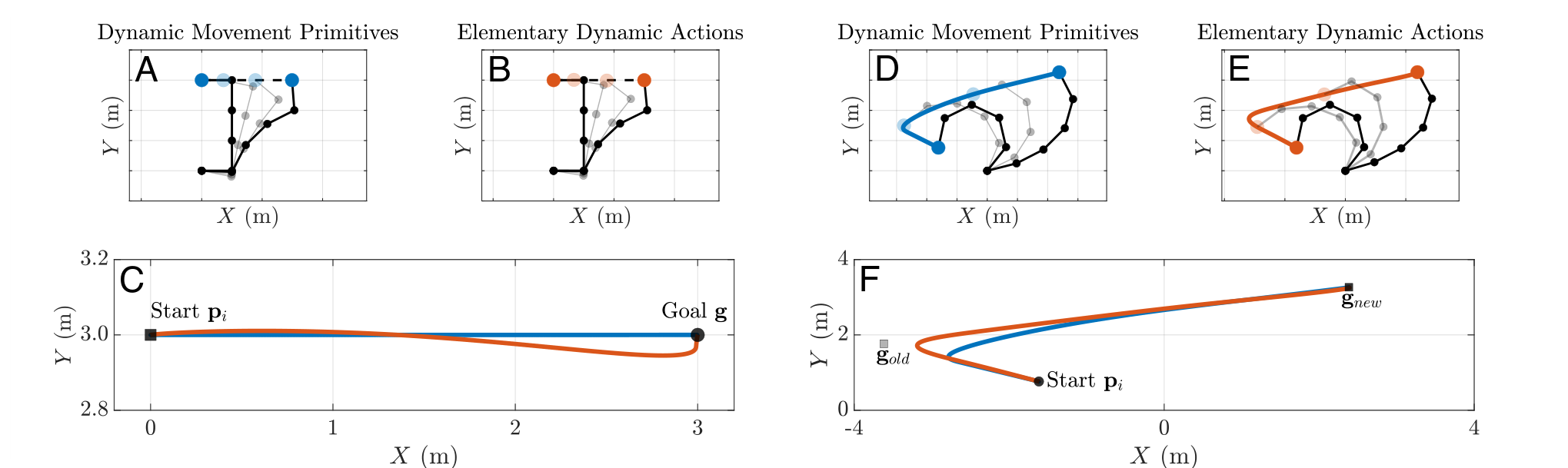
Fig. 11: Managing kinematic redundancy using Dynamic Movement Primitives (DMPs, blue) and Elementary Dynamic Actions (EDAs, orange) (Section 3.9.3). (A, B, C) A single of discrete movement. (D, E, F) A sequence of discrete movements. The first movement headed toward (square grey marker), but at time , target switched location to (square black marker) which necessitated a second movement.
(A, B) The dashed black lines are a minimum-jerk trajectory. (C, F) End-effector trajectories. (A, B, C) Parameters of the minimum-jerk trajectory: m, m, s. (D, E, F) Parameters of the minimum-jerk trajectories: m, m, m, s, s, .
Parameters of DMPs: , , . Other parameters are identical to those in Figure 3. Parameters of EDAs: N/m, Ns/m, Nms/rad.
3.9.2 Elementary Dynamic Actions
Task-space impedance is combined with joint damping to suppress otherwise uncontrolled joint motion. No explicit inverse kinematics is needed. Repetitive motion can still drift in joint space; adding stiffness may control drift but can conflict with the task objective. Superposition must therefore be designed with those tradeoffs in mind.
Equation 22
(22)
3.9.3 Simulation Example
A five-link planar arm performs single and sequential reaches with both controllers. The EDA implementation reuses the previous task impedance and adds joint damping, illustrating modular reuse. The DMP implementation uses its generated reference with the more elaborate feedback mapping.
4 Discussion
The discussion separates shared modular principles from differences in the chosen trajectory and interaction-control implementations.
4.1 Similarities between the Two Approaches
Both approaches reduce motion design to reusable modules and parameters. Shared DMP phase coordinates many joints, while EDA submovements and impedance components simplify combined tasks. Their modularity concerns different mathematical objects, so reuse does not imply identical composition rules.
4.2 Differences between the Two Approaches
The main tradeoffs concern model requirements, tracking, interaction dynamics, singularities, and the level at which modules combine.
4.2.1 The Need for an Inverse Dynamics Model
Inverse dynamics is central to the torque-tracking DMP implementation examined here, while joint-position-controlled robots can execute DMP references through existing servos. Position control alone, however, does not expose the interaction dynamics needed for compliant contact. The comparison should separate the trajectory generator from the robot’s low-level actuation and controller.
4.2.2 Tracking Control
DMPs provide a convenient learned reference for accurate tracking under ideal conditions. EDAs prioritize the impedance relation and need suitable virtual trajectories, impedance choices, or optimization if precise motion tracking is also required.
4.2.3 Contact and Physical Interaction
EDAs treat physical interaction dynamics as an explicit primitive; DMP implementations can add comparable impedance feedback. A PD equation and a first-order joint impedance coincide only with ideal torque sources, and general impedance control can act at other interaction ports.
4.2.4 Managing Kinematic Singularity and Redundancy
Jacobian-transpose impedance commands avoid singular inverses, but do not remove all motion-design concerns. Pseudoinverse-based DMP tracking needs singularity handling and can lose passivity with added null-space projections. Stability claims depend on the complete controller, not just the primitive’s label.
4.2.5 Modularity in Robot Control
EDA virtual trajectories and compatible impedance components admit direct superposition. DMP weights are reusable, but combining distinct motions requires an explicit coordination rule rather than simply merging weight vectors. This distinction explains the sequencing and mixed-motion examples.
4.3 Combining the Best of Both Approaches
Hybrid designs can use DMPs to learn rich virtual trajectories and impedance control to regulate interaction, or add impedance feedback to inverse-dynamics tracking. The paper points to prior variable-impedance learning as an example rather than introducing a newly evaluated hybrid algorithm.
5 Conclusion
The eight simulations clarify tradeoffs between learned trajectory generation and explicit interaction control. They support informed controller design under known assumptions, but provide no physical validation, broad performance ranking, or unconditional safety guarantee.
Acknowledgements
Funding
The work acknowledges MIT/SUSTech research support and a MathWorks fellowship for Moses C. Nah.
Declaration of Conflicting Interests
The authors declare no conflicting interests.
119 references
Abu-Dakka et al. (2015)
Abu-Dakka FJ, Nemec B, Jørgensen JA, Savarimuthu TR, Krüger N and Ude A
(2015) Adaptation of manipulation skills in physical contact with the
environment to reference force profiles.
Autonomous Robots 39: 199–217.
Albu-Schaffer et al. (2003)
Albu-Schaffer A, Ott C, Frese U and Hirzinger G (2003) Cartesian impedance
control of redundant robots: recent results with the DLR-light-weight-arms.
IEEE International Conference on Robotics and Automation :
3704–3709.
Andrews and Hogan (1983)
Andrews JR and Hogan N (1983) Impedance control as a framework for
implementing obstacle avoidance in a manipulator.
Master’s Thesis, M. I. T., Dept. of Mechanical Engineering.
Arimoto (1984)
Arimoto S (1984) Stability and robustness of pid feedback control for robot
manipulators of sensory capability.
In: Robotics Research, 1st Int. Symp.MIT press, pp. 783–799.
Arimoto et al. (2005a)
Arimoto S, Hashiguchi H and Ozawa R (2005a) A simple control
method coping with a kinematically ill-posed inverse problem of redundant
robots: Analysis in case of a handwriting robot.
Asian Journal of Control 7(2): 112–123.
Arimoto and Sekimoto (2006)
Arimoto S and Sekimoto M (2006) Human-like movements of robotic arms with
redundant dofs: virtual spring-damper hypothesis to tackle the bernstein
problem.
In: Proceedings 2006 IEEE International Conference on Robotics
and Automation, 2006. ICRA 2006.IEEE, pp. 1860–1866.
Arimoto et al. (2005b)
Arimoto S, Sekimoto M, Hashiguchi H and Ozawa R (2005b) Natural
resolution of ill-posedness of inverse kinematics for redundant robots: A
challenge to bernstein’s degrees-of-freedom problem.
Advanced Robotics 19(4): 401–434.
Atkeson et al. (2000)
Atkeson CG, Hale JG, Pollick F, Riley M, Kotosaka S, Schaul S, Shibata T,
Tevatia G, Ude A and Vijayakumar S (2000) Using humanoid robots to study
human behavior.
IEEE Intelligent Systems and their applications 15(4): 46–56.
Buchli et al. (2011)
Buchli J, Stulp F, Theodorou E and Schaal S (2011) Learning variable impedance
control.
The International Journal of Robotics Research 30(7):
820–833.
Burdet et al. (2001)
Burdet E, Osu R, Franklin DW, Milner TE and Kawato M (2001) The central nervous
system stabilizes unstable dynamics by learning optimal impedance.
Nature 414(6862): 446–449.
Caccavale et al. (1998)
Caccavale F, Siciliano B and Villani L (1998) Quaternion-based impedance with
nondiagonal stiffness for robot manipulators.
In: Proceedings of the 1998 American Control Conference. ACC
(IEEE Cat. No. 98CH36207), volume 1. IEEE, pp. 468–472.
Chiaverini et al. (1994)
Chiaverini S, Siciliano B and Egeland O (1994) Review of the damped
least-squares inverse kinematics with experiments on an industrial robot
manipulator.
IEEE Transactions on control systems technology 2(2):
123–134.
Chung and Slotine (2009)
Chung SJ and Slotine JJE (2009) Cooperative robot control and concurrent
synchronization of lagrangian systems.
IEEE transactions on Robotics 25(3): 686–700.
d’Avella et al. (2003)
d’Avella A, Saltiel P and Bizzi E (2003) Combinations of muscle synergies in
the construction of a natural motor behavior.
Nature neuroscience 6(3): 300–308.
De Santis et al. (2008)
De Santis A, Siciliano B, De Luca A and Bicchi A (2008) An atlas of physical
human–robot interaction.
Mechanism and Machine Theory 43(3): 253–270.
Degallier et al. (2007)
Degallier S, Righetti L and Ijspeert A (2007) Hand placement during quadruped
locomotion in a humanoid robot: A dynamical system approach.
In: 2007 IEEE/RSJ International Conference on Intelligent
Robots and Systems. IEEE, pp. 2047–2052.
Degallier et al. (2008)
Degallier S, Righetti L, Natale L, Nori F, Metta G and Ijspeert A (2008) A
modular bio-inspired architecture for movement generation for the infant-like
robot icub.
In: 2008 2nd IEEERAS & EMBS International Conference on
Biomedical Robotics and Biomechatronics. IEEE, pp. 795–800.
Degallier et al. (2006)
Degallier S, Santos CP, Righetti L and Ijspeert A (2006) Movement generation
using dynamical systems: a humanoid robot performing a drumming task.
In: 2006 6th IEEE-RAS International Conference on Humanoid
Robots. IEEE, pp. 512–517.
Dietrich and Ott (2019)
Dietrich A and Ott C (2019) Hierarchical impedance-based tracking control of
kinematically redundant robots.
IEEE Transactions on Robotics 36(1): 204–221.
Dietrich et al. (2015)
Dietrich A, Ott C and Albu-Schäffer A (2015) An overview of null space
projections for redundant, torque-controlled robots.
The International Journal of Robotics Research 34(11):
1385–1400.
Elliott et al. (2001)
Elliott D, Helsen WF and Chua R (2001) A century later: Woodworth’s (1899)
two-component model of goal-directed aiming.
Psychological bulletin 127(3): 342.
Flash and Henis (1991)
Flash T and Henis E (1991) Arm trajectory modifications during reaching towards
visual targets.
Journal of cognitive Neuroscience 3(3): 220–230.
Flash and Hochner (2005)
Flash T and Hochner B (2005) Motor primitives in vertebrates and invertebrates.
Current opinion in neurobiology 15(6): 660–666.
Flash and Hogan (1985)
Flash T and Hogan N (1985) The coordination of arm movements: an experimentally
confirmed mathematical model.
Journal of neuroscience 5(7): 1688–1703.
Giszter and Hart (2013)
Giszter SF and Hart CB (2013) Motor primitives and synergies in the spinal cord
and after injury—the current state of play.
Annals of the New York Academy of Sciences 1279(1): 114–126.
Giszter et al. (1993)
Giszter SF, Mussa-Ivaldi FA and Bizzi E (1993) Convergent force fields
organized in the frog’s spinal cord.
Journal of neuroscience 13(2): 467–491.
Haarnoja et al. (2018)
Haarnoja T, Zhou A, Abbeel P and Levine S (2018) Soft actor-critic: Off-policy
maximum entropy deep reinforcement learning with a stochastic actor.
In: International conference on machine learning. PMLR, pp.
1861–1870.
Hermus et al. (2021)
Hermus J, Lachner J, Verdi D and Hogan N (2021) Exploiting redundancy to
facilitate physical interaction.
IEEE Transactions on Robotics 38(1): 599–615.
Hjorth et al. (2020)
Hjorth S, Lachner J, Stramigioli S, Madsen O and Chrysostomou D (2020) An
energy-based approach for the integration of collaborative redundant robots
in restricted work environments.
In: 2020 IEEE/RSJ International Conference on Intelligent
Robots and Systems (IROS). IEEE, pp. 7152–7158.
Hoffmann et al. (2009)
Hoffmann H, Pastor P, Park DH and Schaal S (2009) Biologically-inspired
dynamical systems for movement generation: Automatic real-time goal
adaptation and obstacle avoidance.
In: 2009 IEEE International Conference on Robotics and
Automation. IEEE, pp. 2587–2592.
Hogan (1985)
Hogan N (1985) Impedance control-an approach to manipulation. i-theory.
ii-implementation. iii-applications.
ASME Journal of Dynamic Systems and Measurement Control B 107:
1–24.
Hogan (1987)
Hogan N (1987) Stable execution of contact tasks using impedance control.
In: Proceedings. 1987 IEEE International Conference on Robotics
and Automation, volume 4. IEEE, pp. 1047–1054.
Hogan and Buerger (2018)
Hogan N and Buerger SP (2018) Impedance and interaction control.
In: Robotics and automation handbook. CRC press, pp. 375–398.
Hogan and Flash (1987)
Hogan N and Flash T (1987) Moving gracefully: quantitative theories of motor
coordination.
Trends in neurosciences 10(4): 170–174.
Hogan and Sternad (2007)
Hogan N and Sternad D (2007) On rhythmic and discrete movements: reflections,
definitions and implications for motor control.
Experimental brain research 181(1): 13–30.
Huh and Sejnowski (2015)
Huh D and Sejnowski TJ (2015) Spectrum of power laws for curved hand movements.
Proceedings of the National Academy of Sciences 112(29):
E3950–E3958.
Ijspeert et al. (2013)
Ijspeert AJ, Nakanishi J, Hoffmann H, Pastor P and Schaal S (2013) Dynamical
movement primitives: learning attractor models for motor behaviors.
Neural computation 25(2): 328–373.
Ijspeert et al. (2001)
Ijspeert AJ, Nakanishi J and Schaal S (2001) Trajectory formation for imitation
with nonlinear dynamical systems.
In: Proceedings 2001 IEEE/RSJ International Conference on
Intelligent Robots and Systems. Expanding the Societal Role of Robotics in
the the Next Millennium (Cat. No. 01CH37180), volume 2. IEEE, pp. 752–757.
Ijspeert et al. (2002)
Ijspeert AJ, Nakanishi J and Schaal S (2002) Movement imitation with nonlinear
dynamical systems in humanoid robots.
In: Proceedings 2002 IEEE International Conference on Robotics
and Automation (Cat. No. 02CH37292), volume 2. IEEE, pp. 1398–1403.
International Organization for Standardization (2016)
International Organization for Standardization (2016) ISO-TS 15066:
Robots and robotic devices: Collaborative robots.
Technical report, International Organization for Standardization.
Jayasinghe et al. (2022)
Jayasinghe SA, Scheidt RA and Sainburg RL (2022) Neural control of stopping and
stabilizing the arm.
Frontiers in Integrative Neuroscience 16.
Khatib (1985)
Khatib O (1985) Real-time obstacle avoidance for manipulators and mobile
robots.
In: Proceedings. 1985 IEEE International Conference on Robotics
and Automation, volume 2. IEEE, pp. 500–505.
Khatib (1986)
Khatib O (1986) The potential field approach and operational space formulation
in robot control.
In: Adaptive and Learning Systems: Theory and Applications.
Springer, pp. 367–377.
Khatib (1995)
Khatib O (1995) Inertial properties in robotic manipulation: An object-level
framework.
The international journal of robotics research 14(1): 19–36.
Klein and Huang (1983)
Klein CA and Huang CH (1983) Review of pseudoinverse control for use with
kinematically redundant manipulators.
IEEE Transactions on Systems, Man, and Cybernetics : 245–250.
Koditschek (1987)
Koditschek D (1987) Exact robot navigation by means of potential functions:
Some topological considerations.
In: Proceedings. 1987 IEEE International Conference on Robotics
and Automation, volume 4. IEEE, pp. 1–6.
Kuindersma et al. (2016)
Kuindersma S, Deits R, Fallon M, Valenzuela A, Dai H, Permenter F, Koolen T,
Marion P and Tedrake R (2016) Optimization-based locomotion planning,
estimation, and control design for the atlas humanoid robot.
Autonomous robots 40: 429–455.
Lachner et al. (2021)
Lachner J, Allmendinger F, Hobert E, Hogan N and Stramigioli S (2021) Energy
budgets for coordinate invariant robot control in physical human–robot
interaction.
The International Journal of Robotics Research 40(8-9):
968–985.
10.1177/02783649211011639.
Lachner et al. (2022)
Lachner J, Allmendinger F, Stramigioli S and Hogan N (2022) Shaping impedances
to comply with constrained task dynamics.
IEEE Transactions on Robotics 38(5): 2750–2767.
10.1109/TRO.2022.3153949.
Liegeois (1977)
Liegeois A (1977) Automatic supervisory control of the configuration and
behavior of multibody mechanisms.
IEEE transactions on systems, man, and cybernetics 7(12):
868–871.
Lillicrap et al. (2015)
Lillicrap TP, Hunt JJ, Pritzel A, Heess N, Erez T, Tassa Y, Silver D and
Wierstra D (2015) Continuous control with deep reinforcement learning.
arXiv preprint arXiv:1509.02971 .
Maciejewski and Klein (1985)
Maciejewski AA and Klein CA (1985) Obstacle avoidance for kinematically
redundant manipulators in dynamically varying environments.
The international journal of robotics research 4(3): 109–117.
Maciejewski and Klein (1988)
Maciejewski AA and Klein CA (1988) Numerical filtering for the operation of
robotic manipulators through kinematically singular configurations.
Journal of Robotic systems 5(6): 527–552.
Mussa-Ivaldi and Bizzi (2000)
Mussa-Ivaldi FA and Bizzi E (2000) Motor learning through the combination of
primitives.
Philosophical Transactions of the Royal Society of London.
Series B: Biological Sciences 355(1404): 1755–1769.
Mussa-Ivaldi and Hogan (1991)
Mussa-Ivaldi FA and Hogan N (1991) Integrable solutions of kinematic redundancy
via impedance control.
The International Journal of Robotics Research 10(5):
481–491.
Nah et al. (2020)
Nah MC, Krotov A, Russo M, Sternad D and Hogan N (2020) Dynamic primitives
facilitate manipulating a whip.
In: 2020 8th IEEERAS/EMBS International Conference for
Biomedical Robotics and Biomechatronics (BioRob). IEEE, pp. 685–691.
Nah et al. (2021)
Nah MC, Krotov A, Russo M, Sternad D and Hogan N (2021) Manipulating a whip in
3d via dynamic primitives.
In: 2021 IEEE/RSJ International Conference on Intelligent
Robots and Systems (IROS). IEEE, pp. 2803–2808.
Nah et al. (2023)
Nah MC, Krotov A, Russo M, Sternad D and Hogan N (2023) Learning to manipulate
a whip with simple primitive actions-a simulation study.
iScience .
Nakamura and Hanafusa (1986)
Nakamura Y and Hanafusa H (1986) Inverse kinematic solutions with singularity
robustness for robot manipulator control.
Journal of dynamic systems, measurement, and control 108(3):
163–171.
Nakanishi et al. (2005)
Nakanishi J, Cory R, Mistry M, Peters J and Schaal S (2005) Comparative
experiments on task space control with redundancy resolution.
In: 2005 IEEE/RSJ International Conference on Intelligent
Robots and Systems. IEEE, pp. 3901–3908.
Nakanishi et al. (2008)
Nakanishi J, Cory R, Mistry M, Peters J and Schaal S (2008) Operational space
control: A theoretical and empirical comparison.
The International Journal of Robotics Research 27(6):
737–757.
Park et al. (2008)
Park DH, Hoffmann H, Pastor P and Schaal S (2008) Movement reproduction and
obstacle avoidance with dynamic movement primitives and potential fields.
In: Humanoids 2008-8th IEEE-RAS International Conference on
Humanoid Robots. IEEE, pp. 91–98.
Park et al. (2017)
Park SW, Marino H, Charles SK, Sternad D and Hogan N (2017) Moving slowly is
hard for humans: limitations of dynamic primitives.
Journal of neurophysiology 118(1): 69–83.
Pastor et al. (2009)
Pastor P, Hoffmann H, Asfour T and Schaal S (2009) Learning and generalization
of motor skills by learning from demonstration.
In: 2009 IEEE International Conference on Robotics and
Automation. IEEE, pp. 763–768.
Pastor et al. (2013)
Pastor P, Kalakrishnan M, Meier F, Stulp F, Buchli J, Theodorou E and Schaal S
(2013) From dynamic movement primitives to associative skill memories.
Robotics and Autonomous Systems 61(4): 351–361.
Pastor et al. (2011)
Pastor P, Righetti L, Kalakrishnan M and Schaal S (2011) Online movement
adaptation based on previous sensor experiences.
In: 2011 IEEE/RSJ International Conference on Intelligent
Robots and Systems. IEEE, pp. 365–371.
Penrose (1955)
Penrose R (1955) A generalized inverse for matrices.
In: Mathematical proceedings of the Cambridge philosophical
society, volume 51. Cambridge University Press, pp. 406–413.
Posa et al. (2014)
Posa M, Cantu C and Tedrake R (2014) A direct method for trajectory
optimization of rigid bodies through contact.
The International Journal of Robotics Research 33(1): 69–81.
Raibert and Craig (1981)
Raibert M and Craig J (1981) Hybrid position/force control of manipulators1.
Journal of Dynamic Systems, Measurement, and Control 102: 127.
Saveriano et al. (2019)
Saveriano M, Franzel F and Lee D (2019) Merging position and orientation motion
primitives.
In: 2019 International Conference on Robotics and Automation
(ICRA). IEEE, pp. 7041–7047.
Schaal (2006)
Schaal S (2006) Dynamic movement primitives-a framework for motor control in
humans and humanoid robotics.
In: Adaptive motion of animals and machines. Springer, pp.
261–280.
Schaal and Atkeson (1998)
Schaal S and Atkeson CG (1998) Constructive incremental learning from only
local information.
Neural computation 10(8): 2047–2084.
Schaal et al. (2007)
Schaal S, Mohajerian P and Ijspeert A (2007) Dynamics systems vs. optimal
control—a unifying view.
Progress in brain research 165: 425–445.
Schaal et al. (2005)
Schaal S, Peters J, Nakanishi J and Ijspeert A (2005) Learning movement
primitives.
In: Robotics research. the eleventh international symposium.
Springer, pp. 561–572.
Schulman et al. (2015)
Schulman J, Levine S, Abbeel P, Jordan M and Moritz P (2015) Trust region
policy optimization.
In: International conference on machine learning. PMLR, pp.
1889–1897.
Siciliano (1990)
Siciliano B (1990) Kinematic control of redundant robot manipulators: A
tutorial.
Journal of intelligent and robotic systems 3(3): 201–212.
Slotine and Li (1987)
Slotine JJE and Li W (1987) On the adaptive control of robot manipulators.
The international journal of robotics research 6(3): 49–59.
Stramigioli (2015)
Stramigioli S (ed.) (2015) Energy-Aware Robotics,
Mathematical Control Theory I, volume 461.
Switzerland: Springer International Publishing.
10.1007/978-3-319-20988-3‗.
Takegaki (1981)
Takegaki M (1981) A new feedback method for dynamic control of manipulators.
Trans. ASME, Ser. G, J. Dynamic Systems, Measurement, and
Control 103(2): 119–125.
Tam et al. (2008)
Tam LM, Chen JH, Chen HK and Tou WMS (2008) Generation of hyperchaos from the
chen–lee system via sinusoidal perturbation.
Chaos, Solitons & Fractals 38(3): 826–839.
Theodorou et al. (2010)
Theodorou E, Buchli J and Schaal S (2010) A generalized path integral control
approach to reinforcement learning.
The Journal of Machine Learning Research 11: 3137–3181.
Todorov et al. (2012)
Todorov E, Erez T and Tassa Y (2012) Mujoco: A physics engine for model-based
control.
In: 2012 IEEE/RSJ international conference on intelligent
robots and systems. IEEE, pp. 5026–5033.
Ude et al. (2014)
Ude A, Nemec B, Petrić T and Morimoto J (2014) Orientation in cartesian
space dynamic movement primitives.
In: 2014 IEEE International Conference on Robotics and
Automation (ICRA). IEEE, pp. 2997–3004.
Vijayakumar and Schaal (2000)
Vijayakumar S and Schaal S (2000) Locally weighted projection regression: An o
(n) algorithm for incremental real time learning in high dimensional space.
In: Proceedings of the seventeenth international conference on
machine learning (ICML 2000), volume 1. Morgan Kaufmann, pp. 288–293.
Viviani and Flash (1995)
Viviani P and Flash T (1995) Minimum-jerk, two-thirds power law, and isochrony:
converging approaches to movement planning.
Journal of Experimental Psychology: Human Perception and
Performance 21(1): 32.
Wada and Kawato (2004)
Wada Y and Kawato M (2004) A via-point time optimization algorithm for complex
sequential trajectory formation.
Neural Networks 17(3): 353–364.
Whitney (1969)
Whitney DE (1969) Resolved motion rate control of manipulators and human
prostheses.
IEEE Transactions on man-machine systems 10(2): 47–53.
Wolpert et al. (2001)
Wolpert DM, Ghahramani Z and Flanagan JR (2001) Perspectives and problems in
motor learning.
Trends in cognitive sciences 5(11): 487–494.
Won et al. (1997)
Won J, Stramigioli S and Hogan N (1997) Comment on “The Equivalence of
Second-Order Impedance Control and Proportional Gain Explicit Force
Control”.
The International Journal of Robotics Research 16(6):
873–875.