Overview
The complete supplementary material covers data construction, implementation, failure cases, sampler comparisons, task-and-motion planning, and learned fields. Project materials are linked from the original paper.
At a glance
Diffusion-CCSP learns reusable diffusion models for individual continuous constraint types and composes their predictions on a factor graph. Shared variables receive contributions from all relevant constraints, allowing a single sampling process to seek placements satisfying containment, collision avoidance, stability, and qualitative spatial relations.
Four simulated domains test new constraint combinations and object counts. An outer task-and-motion planner selects discrete action structures; diffusion supplies continuous pose proposals that external checkers verify. The method improves several difficult compositional cases, but success is empirical and finite-budget sampling neither certifies feasibility nor proves infeasibility.
1 Introduction
Robot placement choices interact: a pose can fit inside a box yet block the gripper or make the stack unstable. Solving each constraint sequentially can require repeated rejection and backtracking. Joint optimization addresses these dependencies, but analytic differentiable formulas are difficult to obtain for some qualitative relations.
The proposed alternative learns local constraint models and composes them at inference. Conditioning variables such as geometry stay fixed, while shared decision variables are denoised together. Reuse is over known constraint types and compatible representations; larger or differently connected graphs need not match the training graphs.
2 Related Work
Scene-level methods such as StructDiffusion [14] generate arrangements under a global condition. Compositional energy models, including Gkanatsios et al. [12], combine learned goals. Diffusion-CCSP uses an explicit constraint graph to combine local geometric, physical, and qualitative relations. Specialized packing systems solve narrower combinations, so the paper does not treat them as equivalent general-purpose baselines.
3 Compositional Diffusion Constraint Solvers
A continuous constraint satisfaction problem separates unknown assignments from fixed conditioning data and specifies which constraint types connect them. Qualitative relations such as “close to” are intended to be learnable from context, although the experiments generate their labels with hand-written rules.
3.1 Formulation and Representation of Constraint Satisfaction Problems
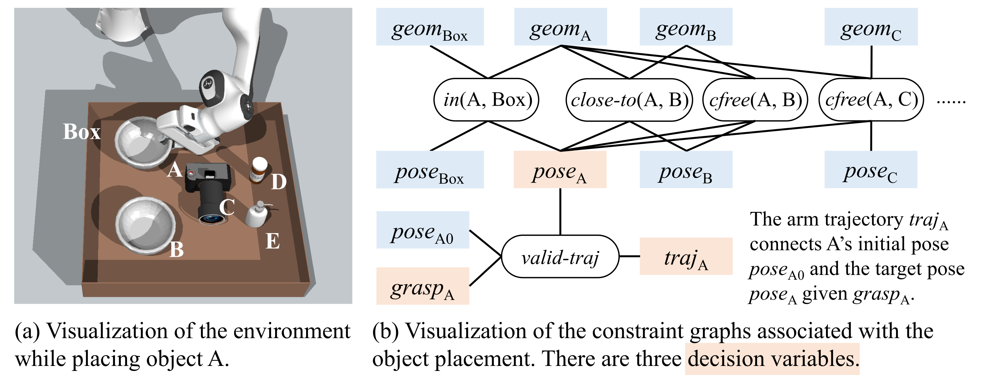
The graph contains decision variables V, conditioning variables U, and typed constraint instances C. Each instance names the variables it consumes. A valid assignment must pass every corresponding test, which may be a rule, classifier, or simulator. “Collision-free” here means nonpenetration.
For a bowl placement, coupled decisions include grasp, target pose, and trajectory. Constraints express containment, proximity to another bowl, collision avoidance, and a valid motion between initial and final poses. This is the general formulation; the robot experiment uses learned pose proposals alongside separate grasp enumeration and motion planning.
Equations
3.2 Compositional Diffusion Models
An ideal component distribution is uniform over the bounded feasible set for one constraint. Multiplying the components corresponds to summing negative-log energies. Annealed unadjusted Langevin sampling combines noisy updates from the learned scores, seeking assignments compatible with all factors. Approximate learned scores and finite sampling do not guarantee an exact product distribution or a valid solution.
Training corrupts a solved graph assignment with Gaussian noise and minimizes the error between that noise and the combined prediction of instantiated constraint modules. Although separate component training is possible, the experiments train the modules jointly on compositional examples. The retained objective and Algorithms 1–2 give the published equations; Algorithm 2 describes the reverse-diffusion update, while the full ULA variant adds the sampling procedure described in Appendix B.
Equations
3.3 Geometric and Physical Constraint Solving with Diffusion-CCSP
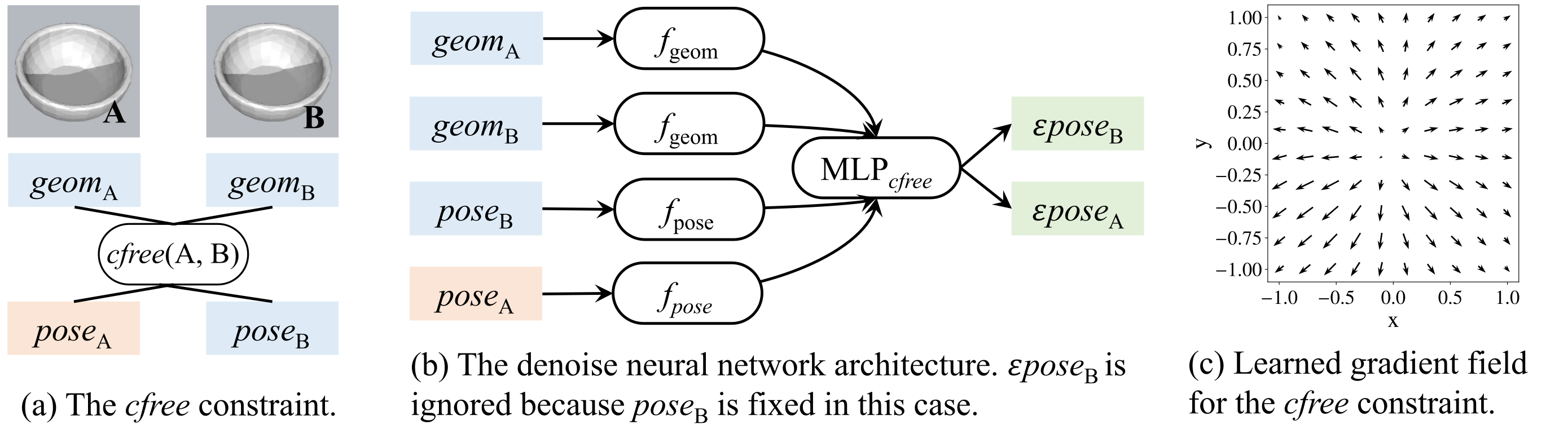
The illustrated network encodes geometry and pose, concatenates the arguments of each constraint with a diffusion-time embedding, and predicts noise for the participating poses. Geometry encoders are shared; pose encoders and interaction modules are constraint-specific. Fixed variables can be conditioned on by discarding their predicted updates.
The general example uses axis-aligned bounding boxes and three-dimensional translation plus yaw, encoded by sine and cosine. The planar tasks use their own compact shape and pose encodings. Point-cloud inputs and arbitrary SE(3) poses are proposed extensions. Figure 3 illustrates a collision-avoidance field, and Appendix F retains all qualitative-field visualizations.
The solver assumes a constraint graph is supplied. Appendix E explains how a symbolic action skeleton generates that graph and how the outer planner retries when sampled continuous assignments fail validation.
Equation
|
|
4 Experiments
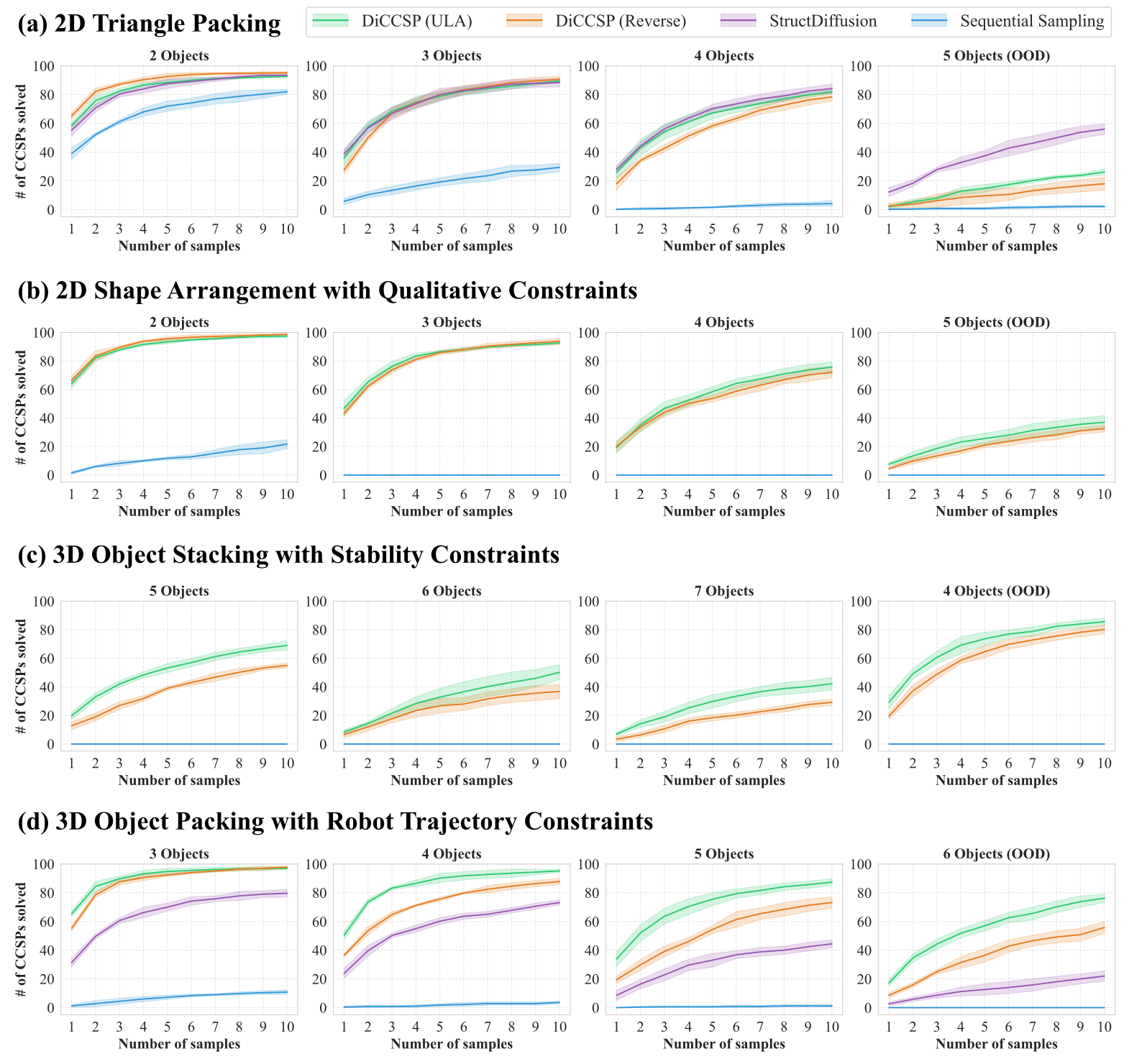
The four tasks compare ULA sampling with direct reverse diffusion, sequential rejection sampling, and a task-adapted StructDiffusion baseline where applicable. Sequential sampling tries at most 50 poses per object. StructDiffusion is tested on triangle packing and robot packing, using a single scene-level constraint. Main success curves count problems solved within ten samples and show variation across five training seeds.
4.1 2D Triangle Packing
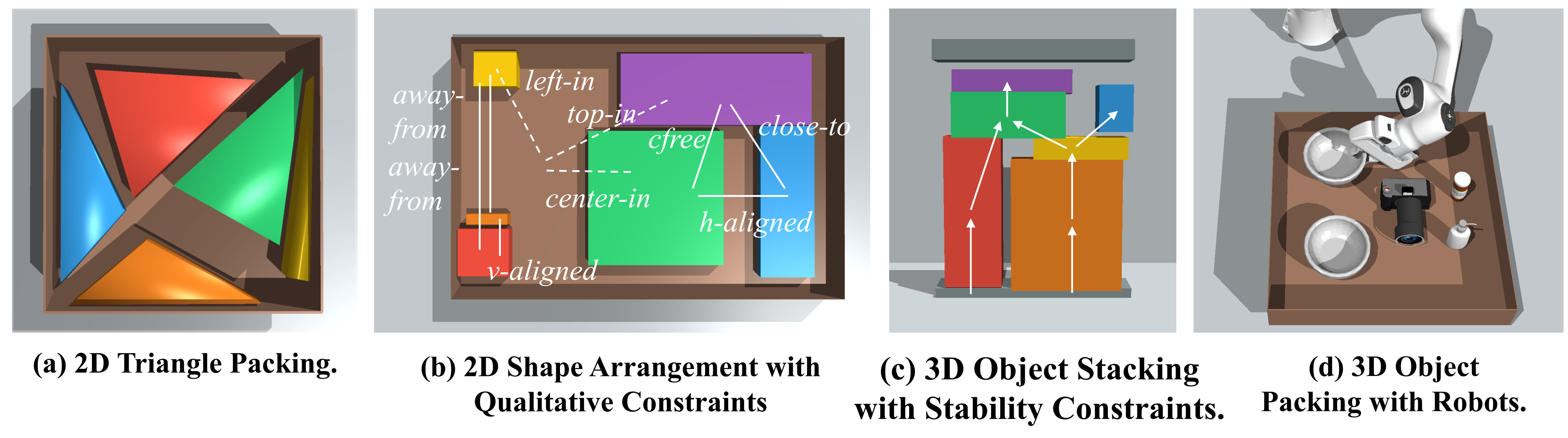
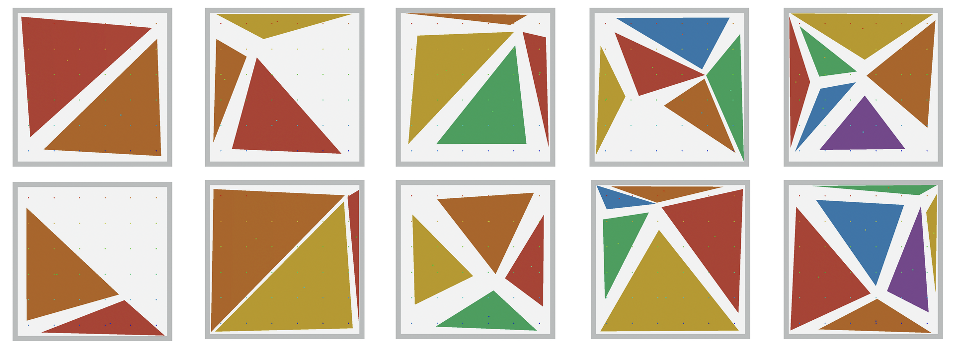
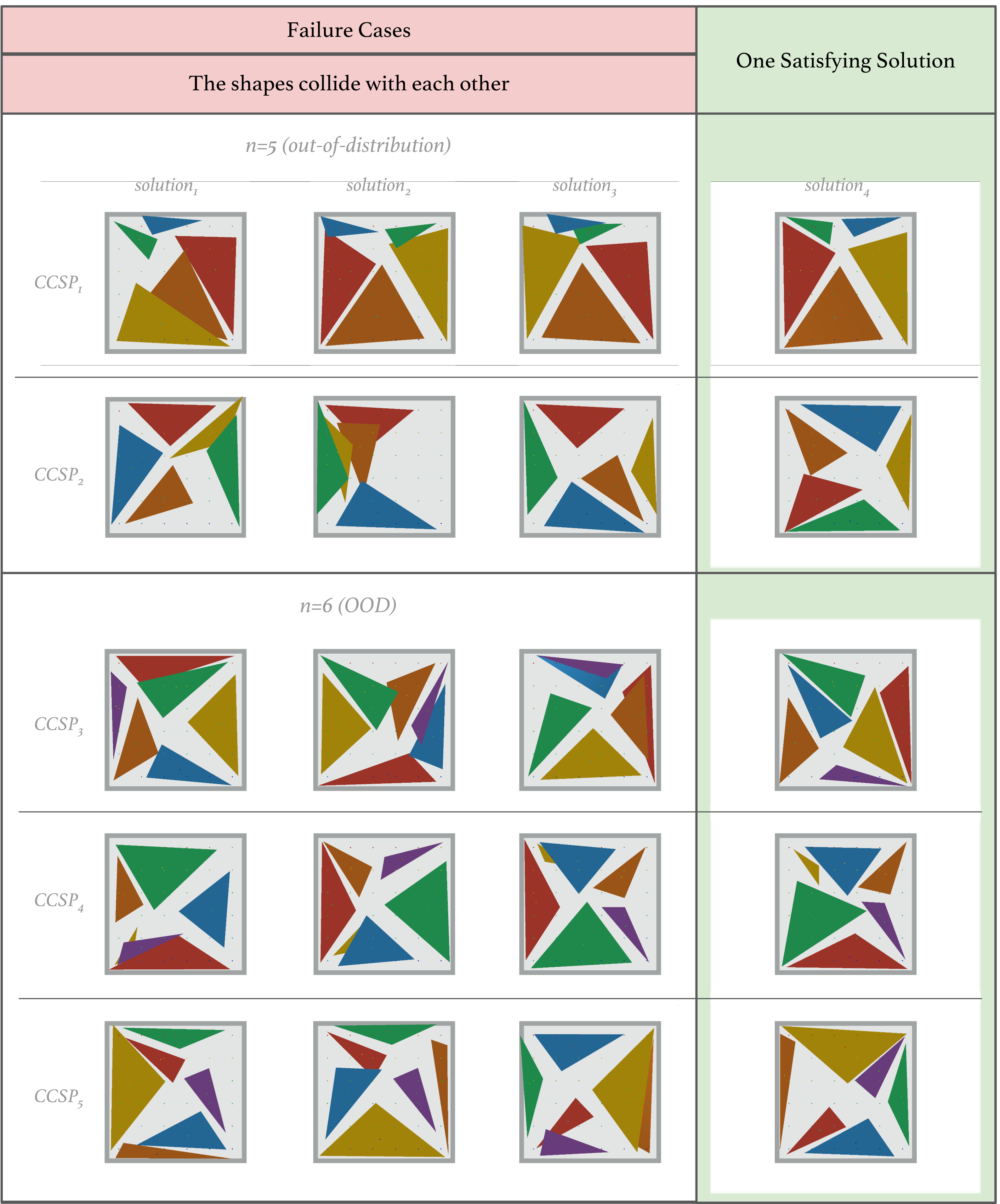
Training uses 30,000 solutions with two to four rotatable triangles; tests include five-triangle problems. Random tray triangulations generate collision-free examples. Rejection sampling becomes weak as packing gets dense. StructDiffusion performs comparably in distribution and generalizes better than Diffusion-CCSP to five triangles, so the compositional model does not dominate every task.
4.2 2D Shape Arrangement with Qualitative Constraints
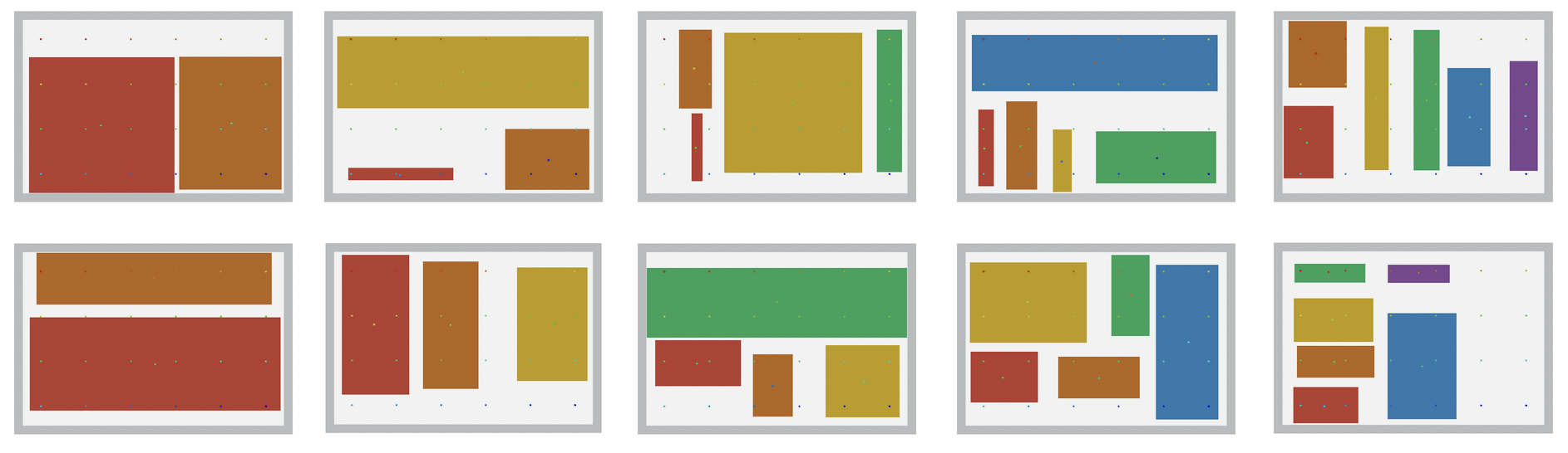
Rectangles must satisfy containment, noncollision, and selected relations such as relative position, proximity, and alignment. Training uses 30,000 two-to-four-object examples. The plotted quantitative test extends to five objects; the illustrative six-object scene contains 45 constraints of 13 types. The text also discusses six-object rejection failure, but that example should not be conflated with the plotted test range.
Diffusion-CCSP outperforms the sequential baseline on these combinations. Success still declines sharply on the five-object distribution shift, and narrow or disconnected feasible regions remain difficult.
4.3 3D Object Stacking with Stability Constraints
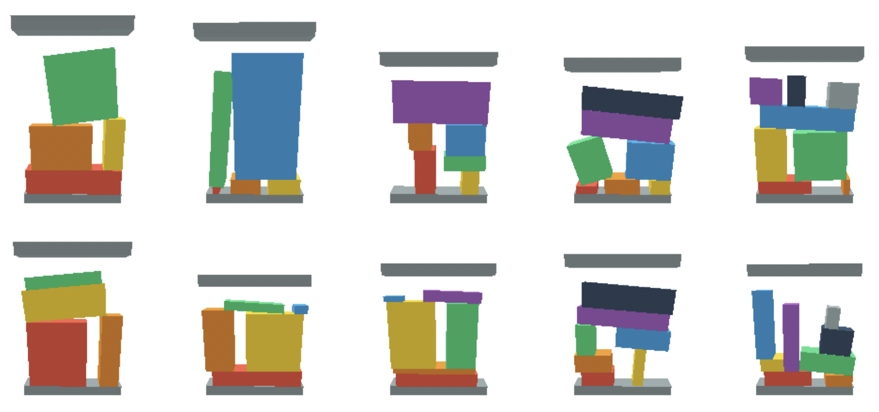
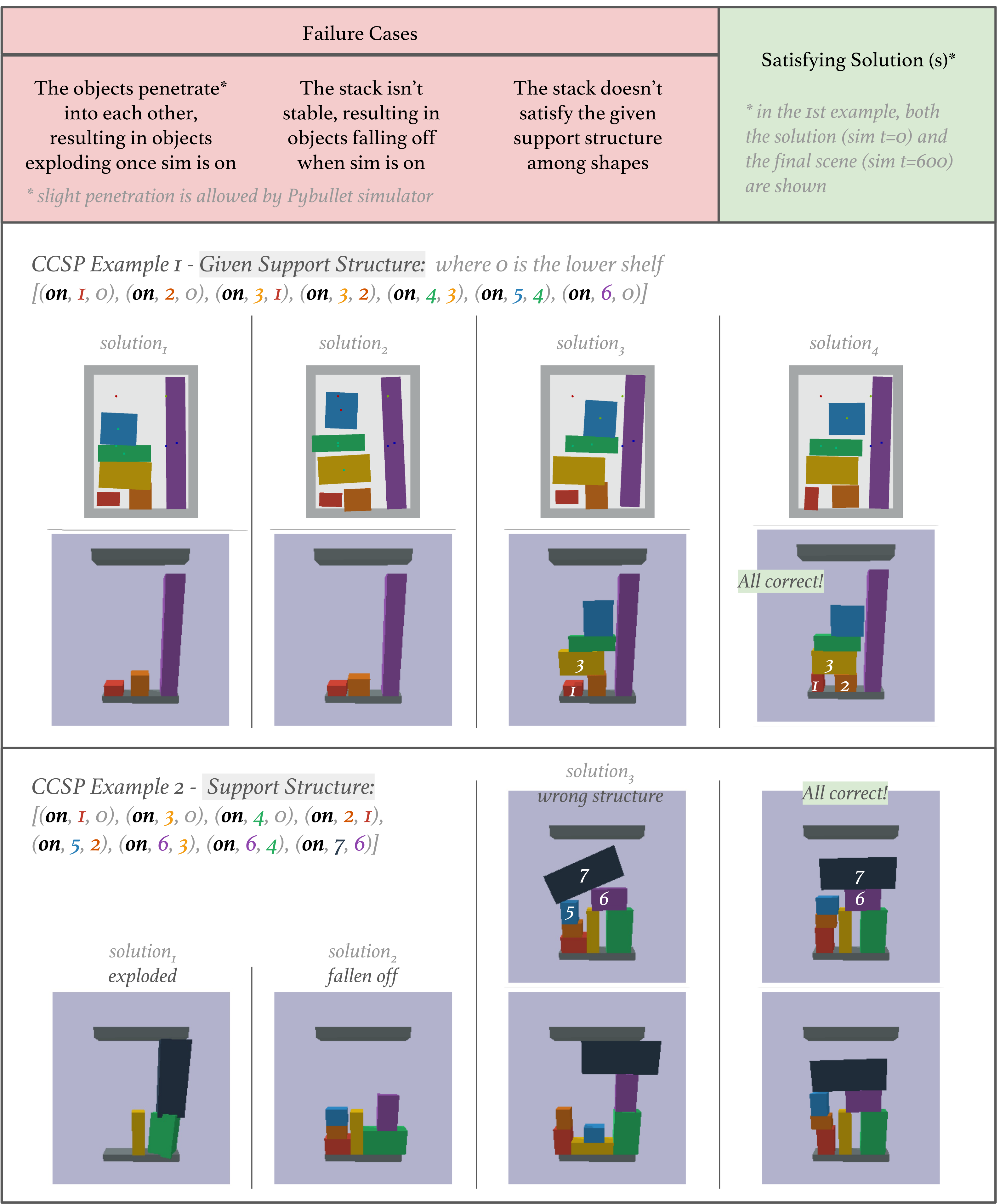
The stacking task places prism-like objects on a shelf under support and stability constraints. Every example contains a bridge supported by multiple objects, and both intermediate placements and the final stack must remain stable. Training uses 24,000 five-to-seven-object examples; evaluation also includes four-object graphs.
An outer planner samples placement orders and support structures before calling the continuous solver. A failed call may reflect an infeasible structure or unsuccessful sampling. Table 1(a) reports 11.9 calls for four objects and 33.33 for five; the narrative’s separate six-object example is not a tabulated measurement. Batched throughput figures are reported separately from complete planning latency.
4.4 Task 4: 3D Object Packing with Robot Trajectory Constraints
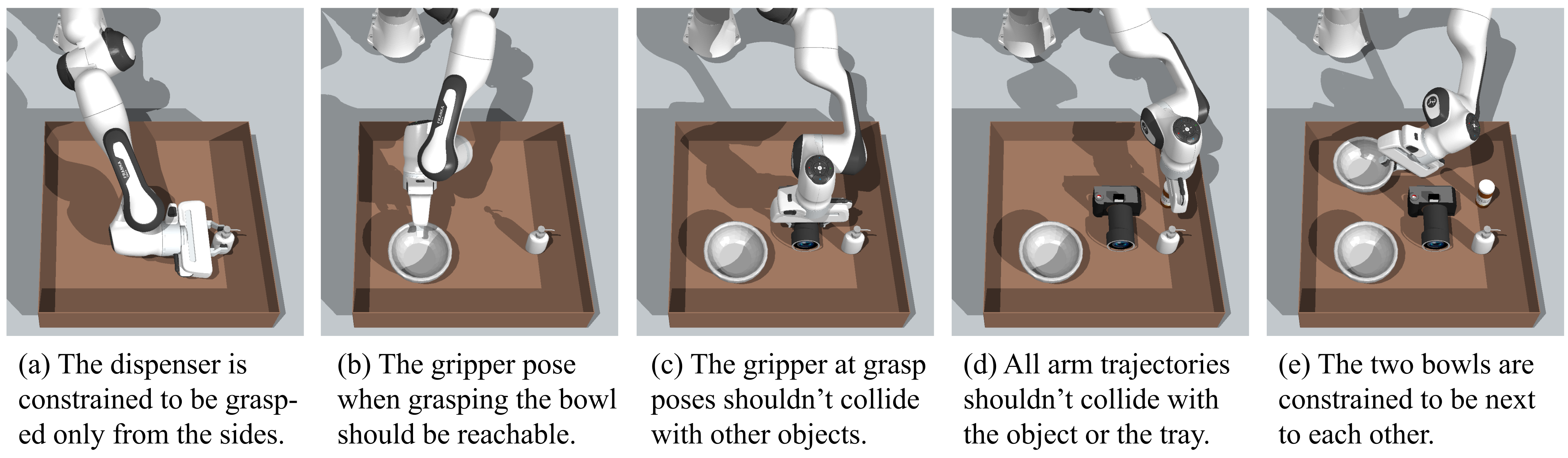
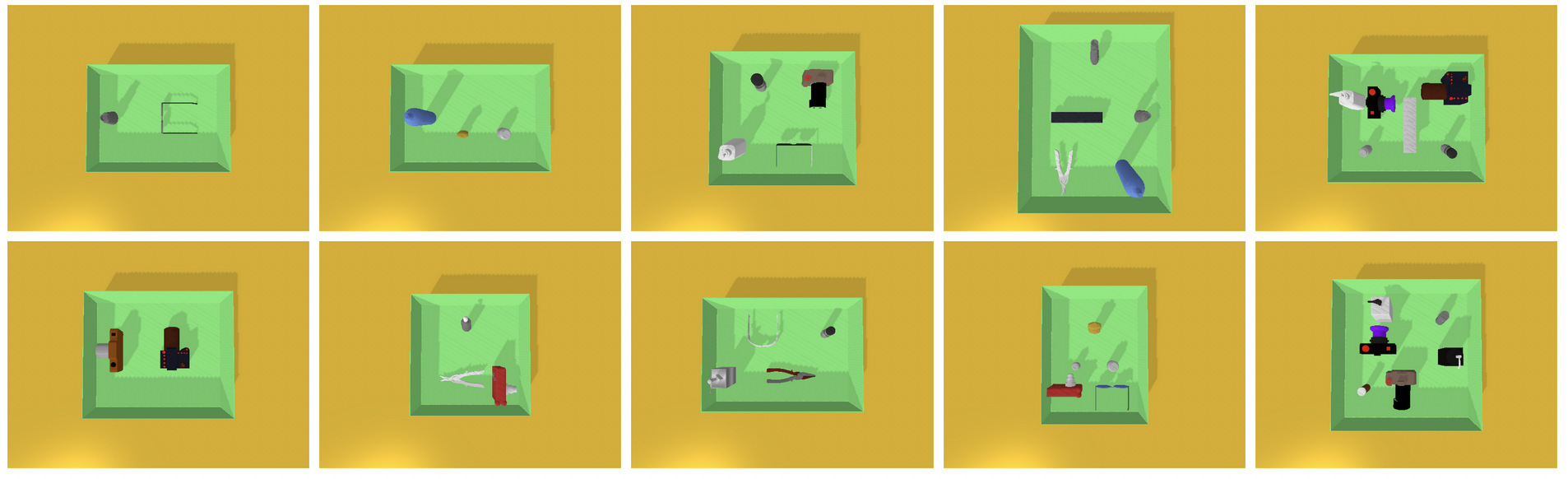
A simulated Franka Panda packs 53 assets from PartNet Mobility and ShapeNet, including 15 assets restricted to side grasps. Training has 10,000 examples with three to five objects, and testing extends to six. Candidate grasps are generated beforehand; an external motion planner checks trajectories.
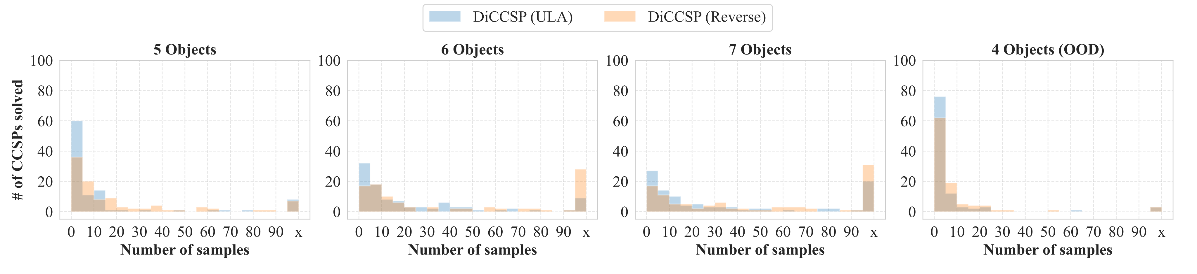
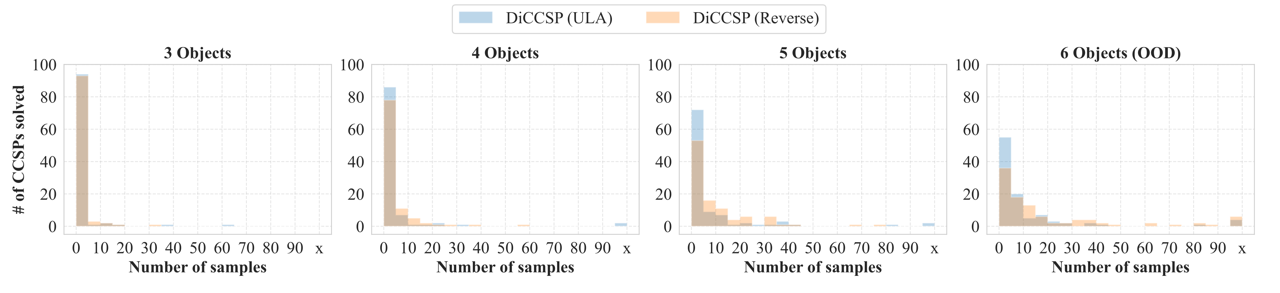
Diffusion predicts placements likely to admit feasible grasps and motions; it does not directly synthesize arm trajectories. Within ten samples, the six-object result is approximately 60–80% across the two diffusion variants, exceeding the listed rejection and StructDiffusion baselines. The source accidentally calls these “six-triangle” cases; Figure 5(d) is the robot-packing experiment. Table 1(b) reports the full planner’s increasing solver-call counts.
5 Limitation and Conclusion
The demonstrated reuse is over fixed-arity known constraints, fully observed states, compact geometry encodings, and simulated rule-labeled examples. Variable-arity factors, natural-language conditioning, richer shapes, and human-derived qualitative labels remain future work. The system also depends on an outer symbolic planner for action order.
The contribution is a modular learned proposal mechanism for continuous assignments that can be inserted into a planning system. It offers useful empirical generalization, while external validity checks and repeated samples remain essential. The authors acknowledge government, university, and industry research support.
Appendix A Problem Domains and Data Generation
The datasets balance examples across their included object counts. Construction starts from satisfiable arrangements, then derives constraints or validates action sequences, which shapes the distribution the models learn.
A.1 2D Triangle Packing
Bowyer–Watson triangulation splits sampled tray points into triangles, which are slightly shrunk to leave clearance. A canonical triangle places one vertex at the origin and its longest incident edge on the positive x-axis. Geometry uses that edge length and the other vertex vector; pose uses translation and sine/cosine rotation.
A.2 2D Shape Arrangement with Qualitative Constraints
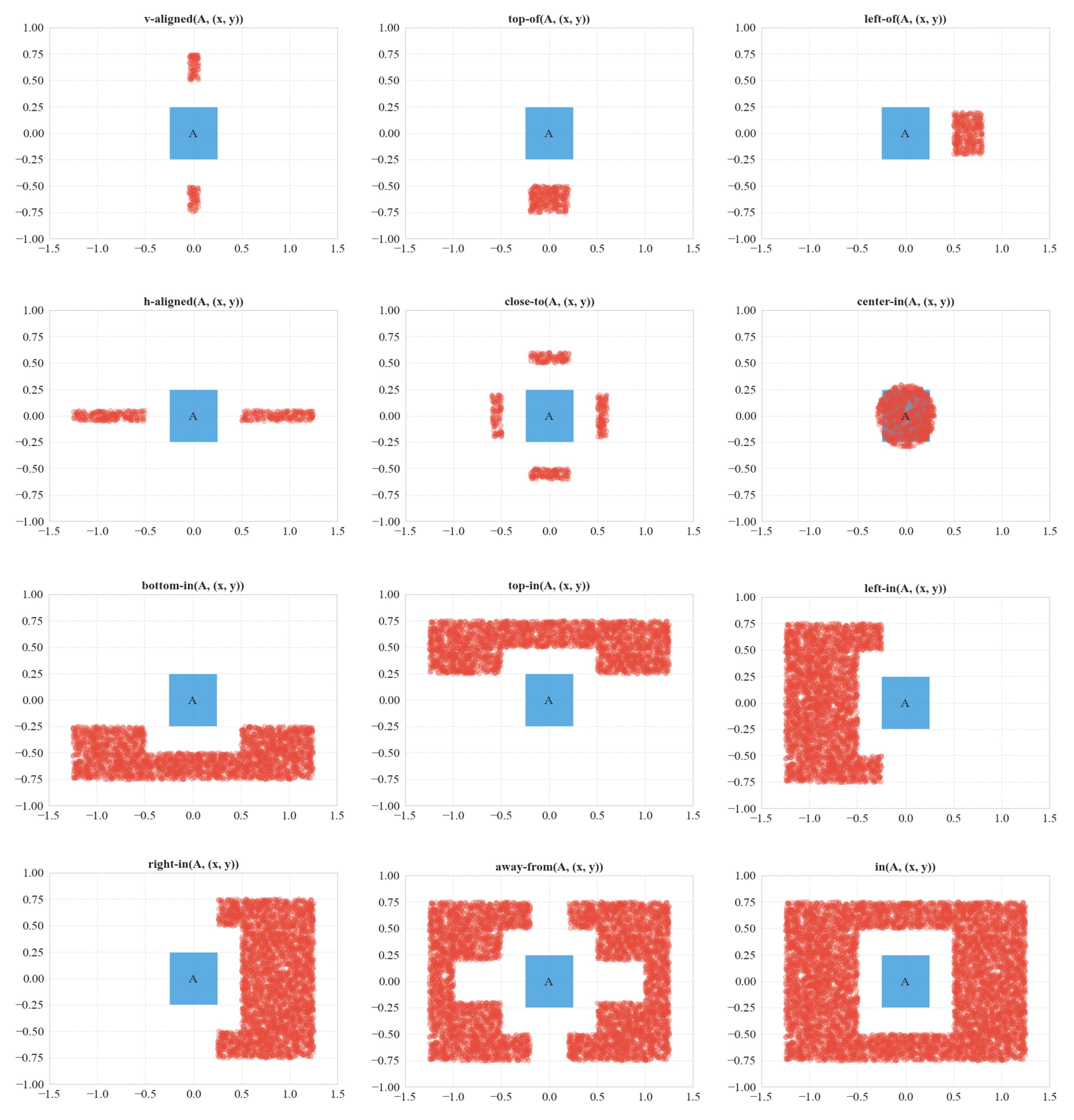
Recursive tray subdivision to depth three generates rectangles, with random padding and rejection of tiny regions. Hand-written rules label eleven qualitative relations; for example, “close to” uses a distance threshold tied to object widths. The full list and sample arrangements remain visible in the figures.
Rectangles use width and length in a horizontal resting pose. Decision variables are centroid position and sine/cosine yaw; some constraint combinations require vertical orientation.
A.3 3D Object Stacking with Stability Constraints
A vertical region is split, shrunk, and cut into shapes that settle in PyBullet. Configurations are retained only if stable, and removing objects one at a time checks stability of intermediate stages. The upper shelf allows only slight clearance. The reported encoding uses width, length, centroid coordinates, and sine/cosine roll, restricting the pose search despite the three-dimensional simulation.
A.4 3D Robot Packing with Robots
The 53 assets span dispensers, bowls, flat staplers, eyeglasses, pliers, scissors, cameras, bottles, opened bottles, and mugs. Prespecified grasps approach one of five object faces. Random tray subdivisions determine object scale and candidate placement regions; a planner checks grasp combinations, collision-free approach poses, and arm paths for a sampled placement order.
Geometry is an object bounding box, grasp is a five-entry face indicator, and placement pose contains tray-frame translation plus sine/cosine yaw. This finite grasp representation is narrower than arbitrary continuous grasp generation.
A.5 Discussion: Sample Complexity of Diffusion-CCSP
Each task needs approximately 10,000–30,000 solved examples. Simulation supplies geometric and physical examples, while realistic qualitative relations would require costly human annotations or another data source. The authors argue that geometric learning should transfer readily, but this paper does not establish sim-to-real performance with physical robot trials.
A.6 Discussion: Partial Observability
All experiments assume known shapes and initial poses. Completing meshes from partial point clouds, detecting collisions during execution, and replanning are suggested ways to relax that assumption; no partial-observation experiment is reported.
Appendix B Implementation and Training Details
Geometry, pose, grasp, and time embeddings have width 256, with inputs normalized relative to the container. A pose decoder maps combined module outputs to predicted noise. The implementation description averages contributions for each object, whereas the main mathematical objective writes a sum; both original descriptions are retained without assuming they are numerically identical.
Most models use 1,000 diffusion timesteps; Diffusion-CCSP uses 500 for robot packing. ULA uses ten sampling steps with step size twice the cosine-scheduled beta. Multiple random seeds are batched for throughput.
The StructDiffusion adaptation concatenates geometry and pose into 512-dimensional tokens, or 768 dimensions with grasp features. It uses four residual attention blocks with two heads and normalization. Language embeddings are omitted because these tasks provide no language input. The rejection baseline samples each object at most 50 times.
B.1 Discussion: Individual Constraint Diffusion Training and Finetuning
Joint training fits the constraint modules through examples containing several simultaneous factors. Independent training and later composition are supported by the formulation but are not the main experimental protocol. Finetuning for new shapes is a proposed use.
B.2 Discussion: Weights for Energy Function Composition
The authors use unit weights for all constraint types. They attribute the workable composition to steep learned fields and joint training on combined constraints. This is an empirical choice, not a guarantee that unit weighting works for arbitrary factors; the separate per-object averaging detail also matters.
B.3 Discussion: Local Optima in Optimization
Parallel initial-noise seeds reduce sensitivity to bad local optima but do not remove it. The cited five-object stacking case averages 33.3 calls. Simulator checks validate collision and stability; learned checkers are suggested when a direct test is unavailable. Repeated invalid samples do not certify an empty feasible set.
Appendix C Failure Case Analysis
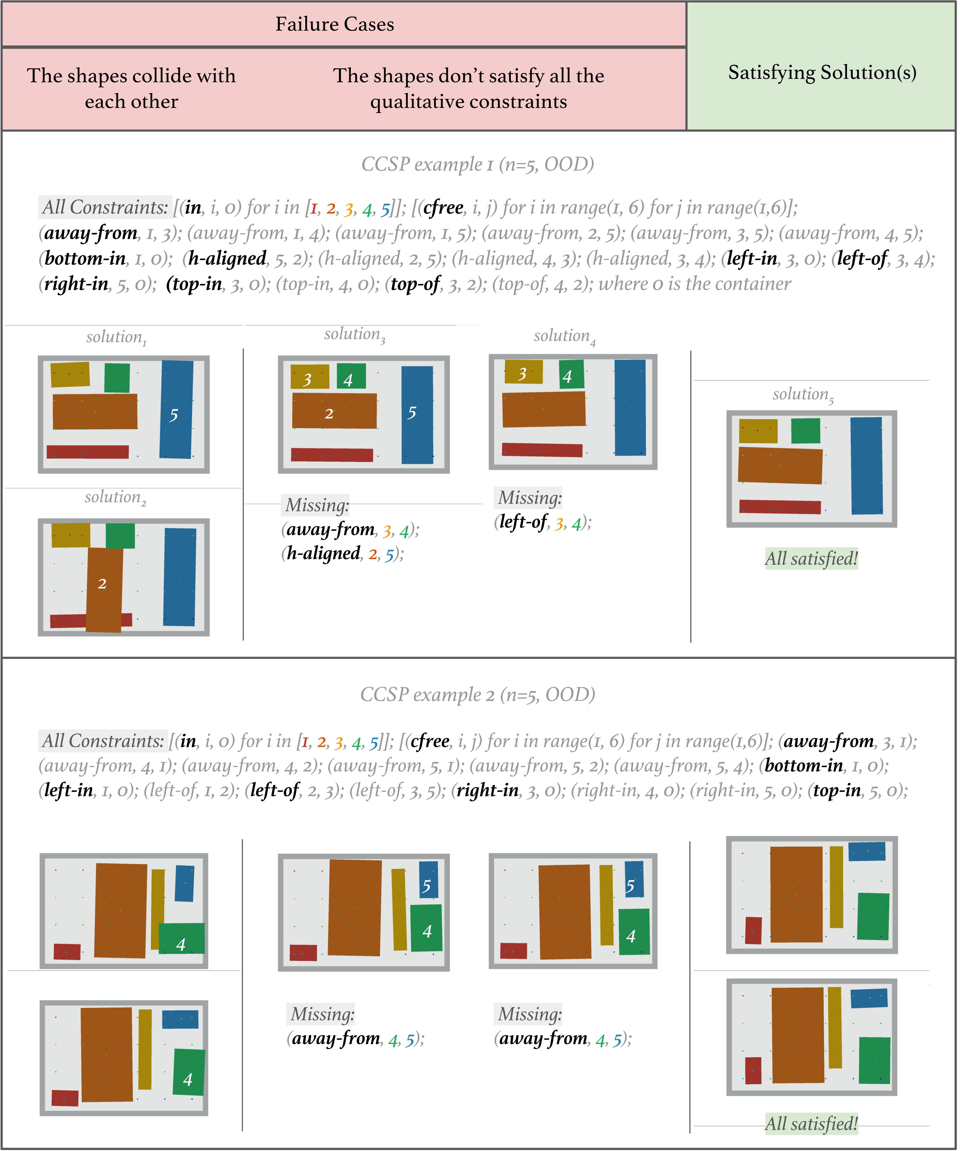
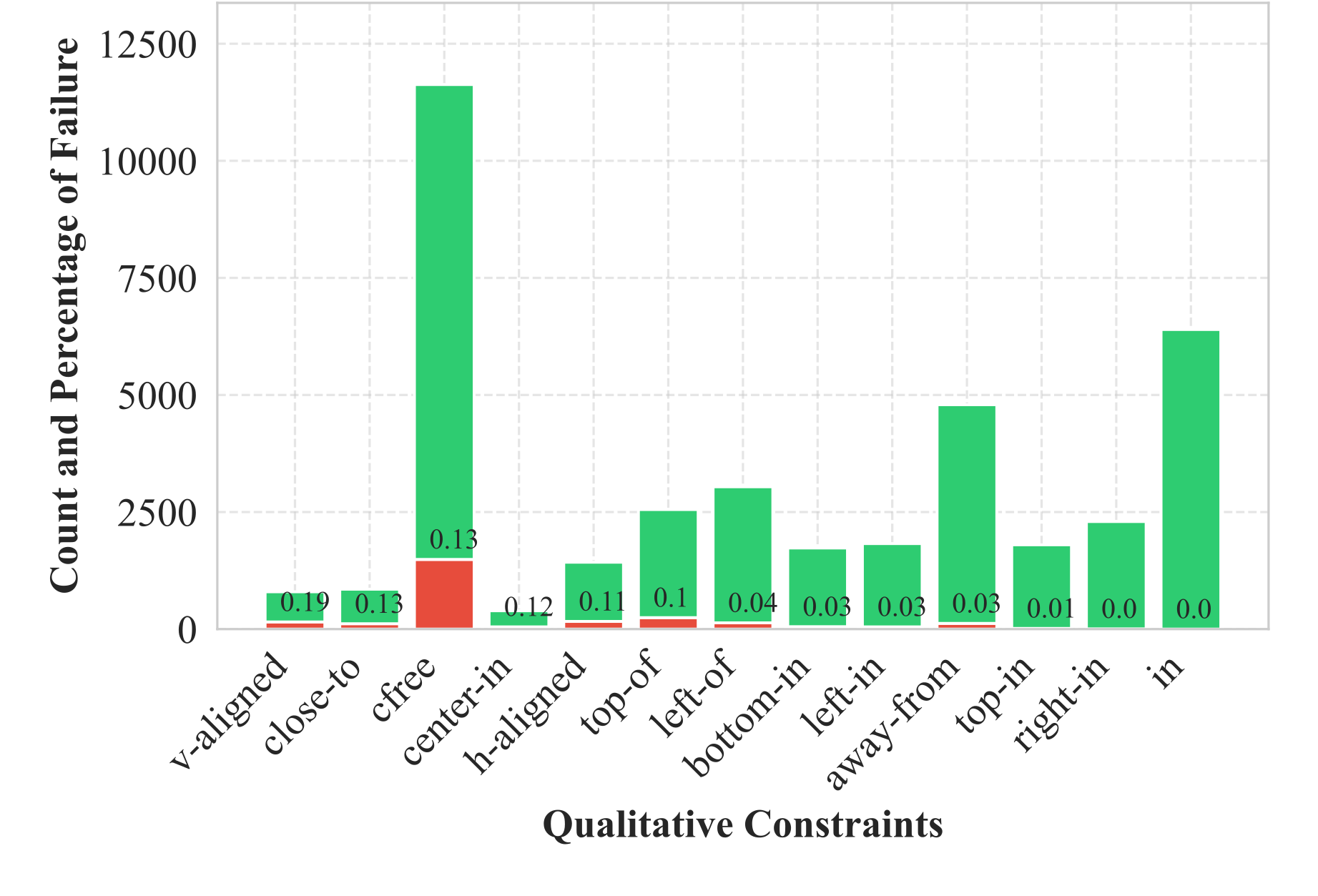
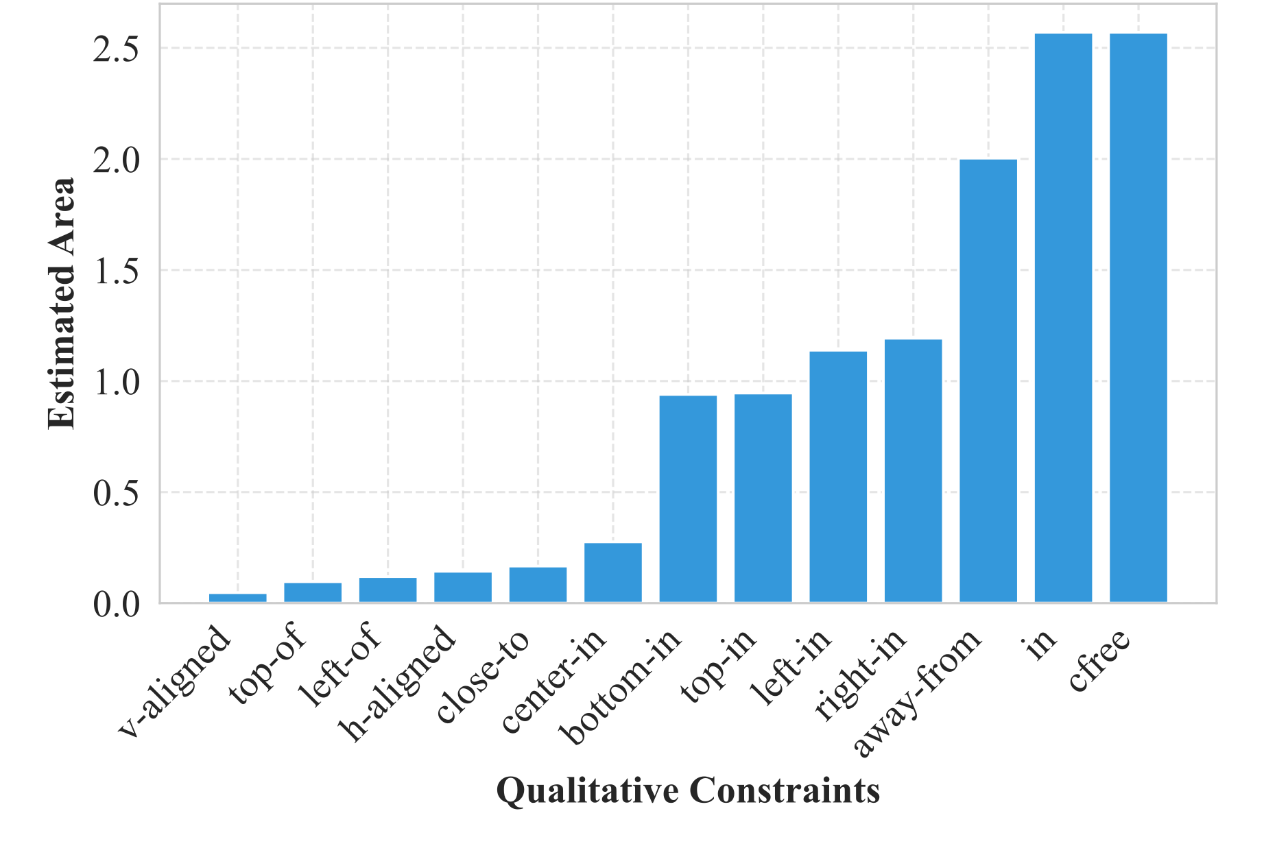
The failure analysis runs 4,000 solver calls on 400 two-to-four-shape qualitative problems. Narrow feasible regions, rare training constraints, and disconnected valid sets correlate with more failures. A separate two-object rejection estimate measures feasible area; it does not characterize multi-object collision-free volume, so collision avoidance is excluded from that particular comparison.
Figures 11–14 retain both failed and successful samples, including triangle overlap, missing qualitative relations, penetration-induced simulator instability, falling stacks, and incorrect support structures. Slight penetration is tolerated by the simulator, as the original figure notes.
Appendix D Additional Sampler Comparison
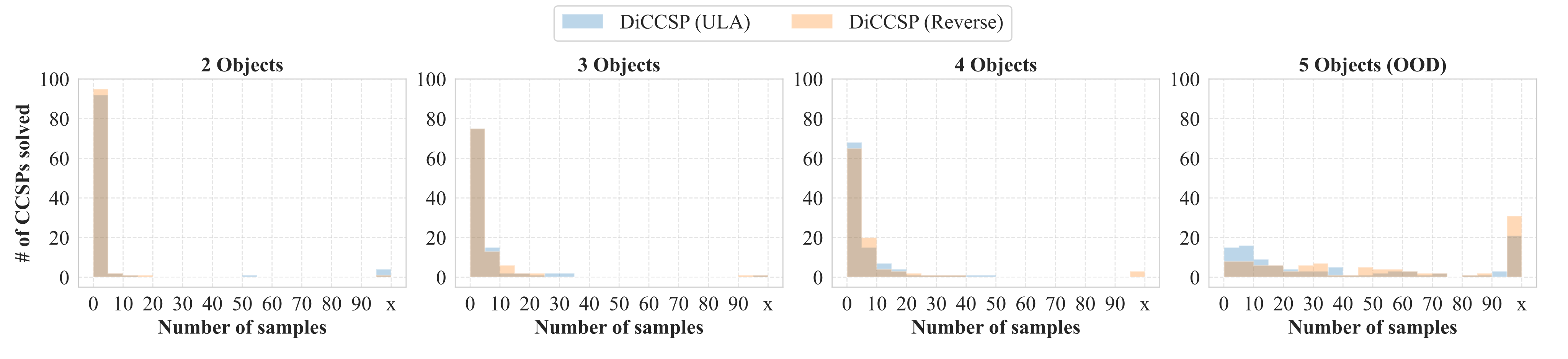
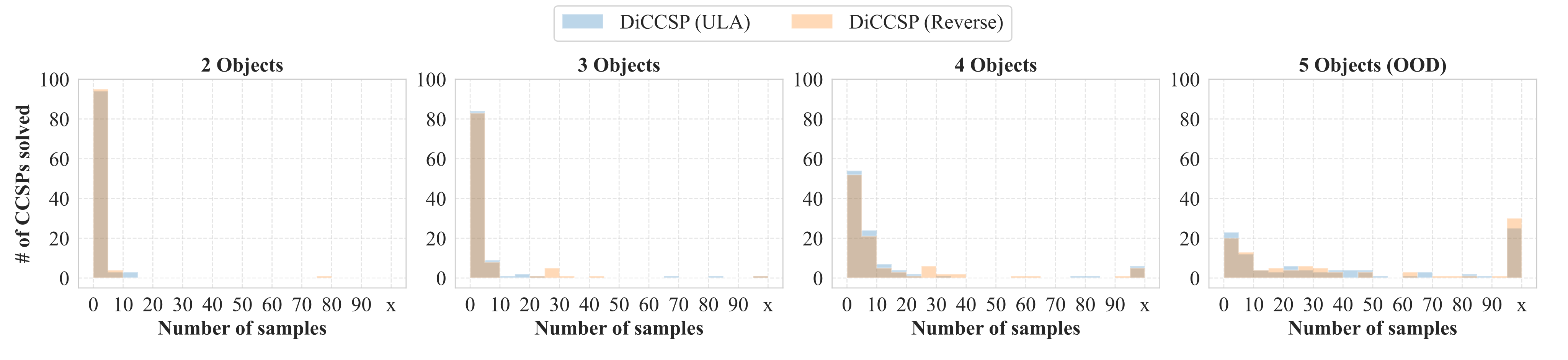
The expanded sampler comparison allows up to 100 samples per problem. Figure 15 includes an explicit unsolved bin, preventing failed cases from disappearing into a mean. Table 2 reports amortized per-problem time in batches of 100: roughly 0.01–0.04 s for reverse diffusion and 0.06–0.19 s for ULA. These are batched sampling costs, not complete robot-plan runtimes.
Appendix E Integration with Task and Motion Planning Algorithms
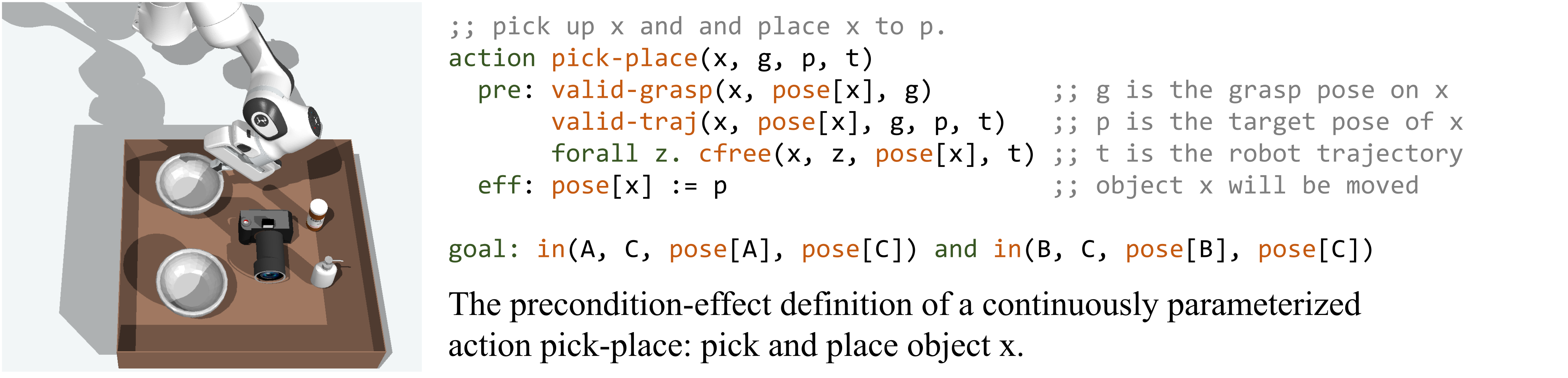
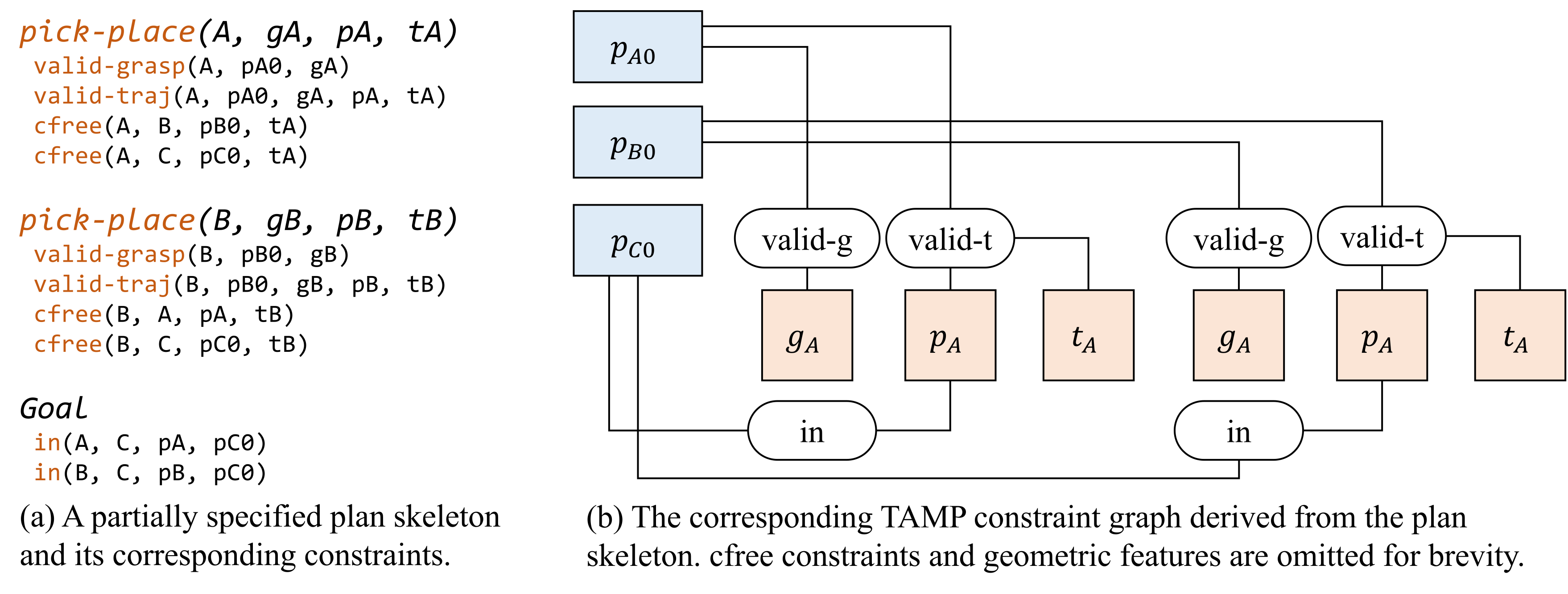
A task-and-motion planning problem specifies initial state, goals, parameterized actions, and a transition model. Action preconditions constrain grasps, placements, and trajectories; effects update the object state. The retained formal semantics and Figures 16–17 show the pick-and-place domain and a two-action constraint graph.
Following the bi-level approach discussed in the TAMP survey [36] and PDDLStream [4], the outer search chooses discrete objects and action order, then a continuous solver proposes the remaining values. A validated assignment instantiates the skeleton; failure prompts another sample or skeleton. The examples use a simplified planner, not a demonstration of solving arbitrary TAMP domains.
Equations
Appendix F Learned Gradient Fields
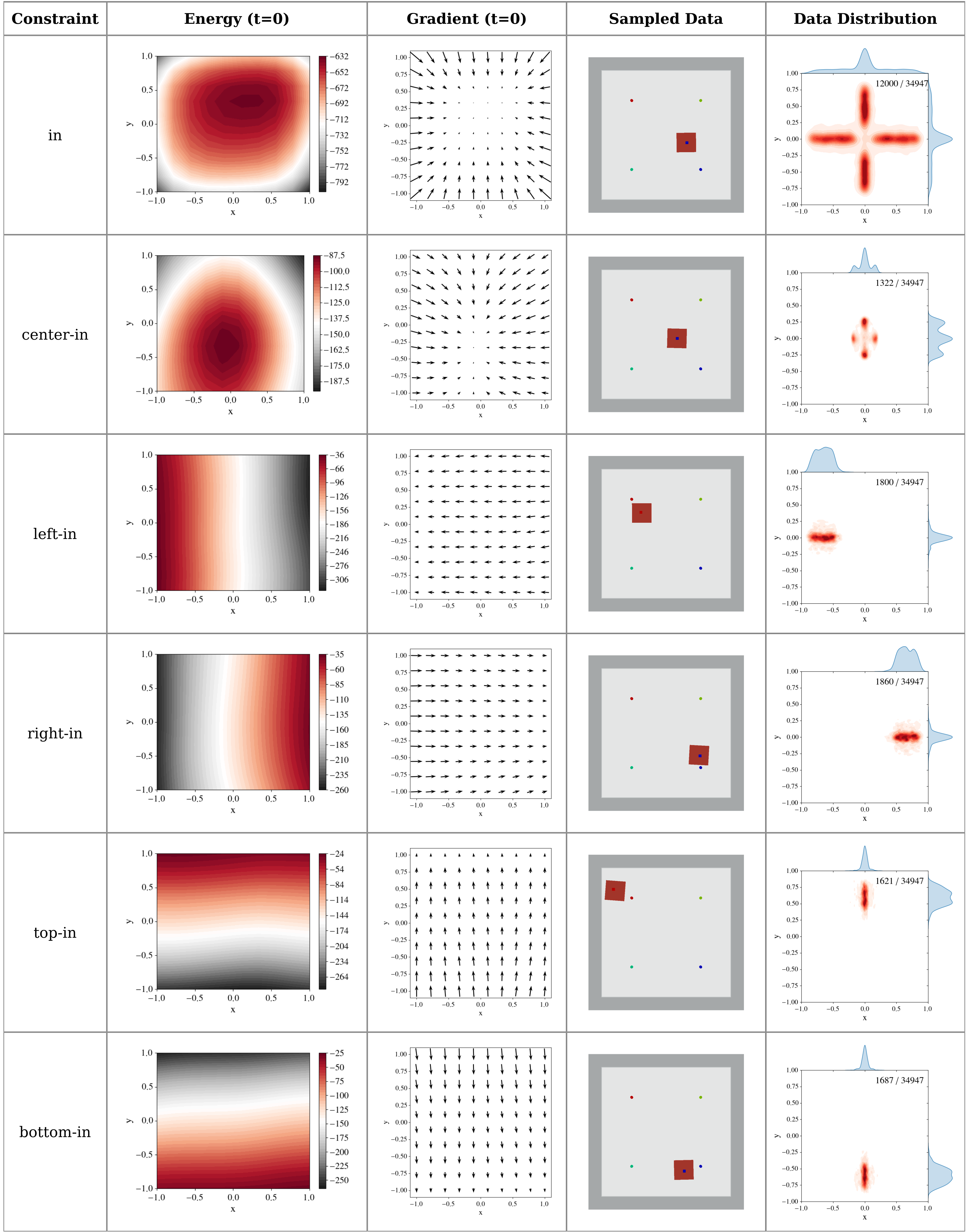
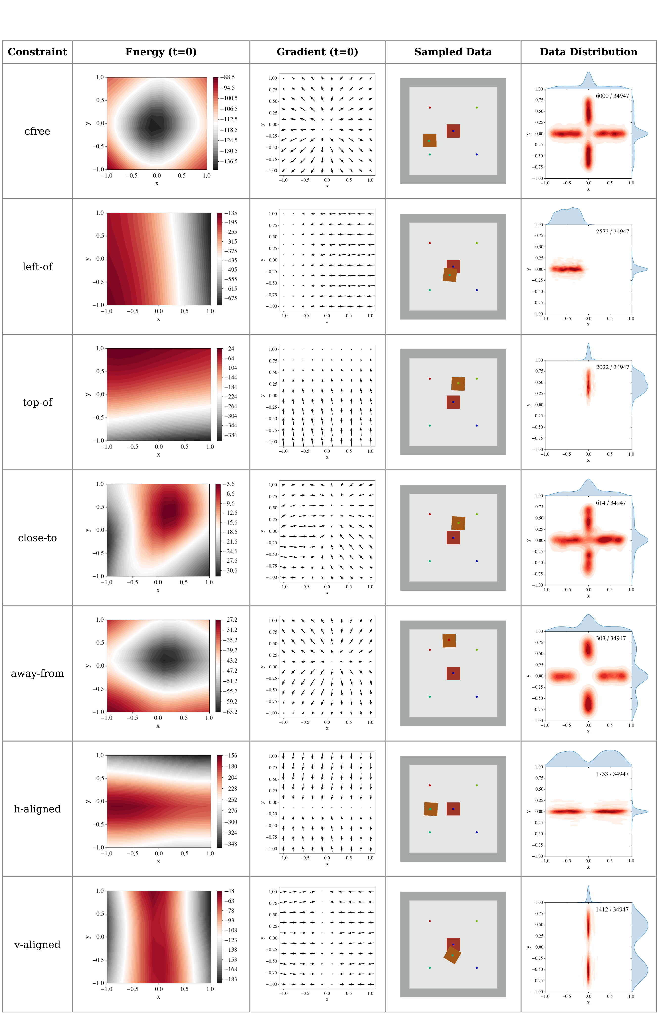
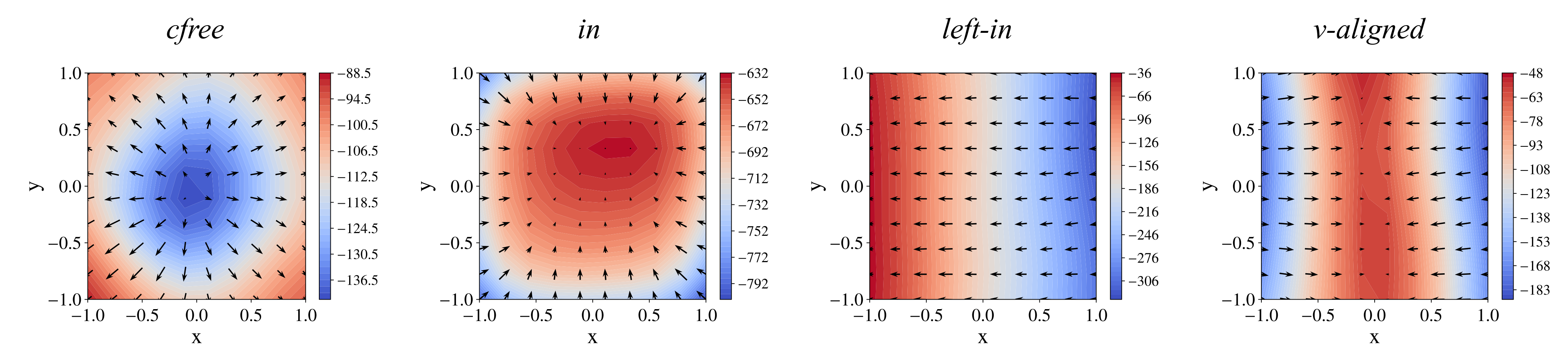
Figures 18–19 show all thirteen geometric and qualitative fields. Unary visualizations move a 0.15 × 0.15 square inside a unit container; binary visualizations fix a second square at the origin. Columns show an energy proxy, update field, sampled pose, and training distribution. The training plots contain different normalized shapes, so they are not identical slices of the visualized test geometry.
The paper constructs its energy visualization from the difference between input noise and reconstructed output at the final diffusion step. These qualitative plots illustrate low-value feasible regions and update directions; they do not independently establish exact calibrated energies or convergence guarantees.