A leader actively chooses its trajectory to reveal which of finitely many known objectives governs a boundedly rational follower. The follower uses a maximum-entropy linear quadratic controller; the leader maximizes separation among its predicted Gaussian state distributions through a difference-of-convex program. In two simulated receding-horizon games, the posterior identifies the true hypothesis faster than a feasible random-trajectory baseline. The evidence is numerical and Gazebo simulation, not human or physical-robot testing.
I Introduction
Passive inverse-game methods infer objectives from already collected behavior. This paper instead chooses actions that make self-interested follower responses informative, without requiring cooperative preference labels. It combines a maximum-entropy game model with finite-hypothesis identification and a convex-concave optimization procedure. The leader already knows the candidate cost/observation models; the task is to distinguish their types online, not discover an arbitrary unknown reward. Human-driver interaction motivates the setup, but demonstrations use synthetic rationality models.
II Linear quadratic Stackelberg trajectory games
Each player controls a stochastic linear time-invariant system. The leader commits to a trajectory; the follower responds by tracking a linear transformation of it while balancing control effort and entropy. This structure makes conditional behavior and state moments analytically tractable.
II-A The dynamics of the players’ systems
Leader and follower states follow separate known linear dynamics with independent, identically distributed, zero-mean Gaussian process disturbances and positive-definite covariances. Their state and input dimensions may differ. In the experiments, double-integrator trajectories approximate ground-rover motion, then a separate controller tracks those references in Gazebo.
Equations 1–3
(1)
(2)
(3)
II-B The players’ objectives
The follower minimizes quadratic tracking error and input effort with a negative log-determinant term that rewards Gaussian action entropy. Proposition 1 supplies backward Riccati-style recursions for its optimal action covariance and affine state-feedback mean, followed by forward recursions for Gaussian state moments. Bounded-rationality noise is part of this assumed probabilistic model, not fitted evidence about actual human behavior.
The leader’s general bilevel objective combines expected joint trajectory cost with an input-only regularizer, subject to follower optimality. The proposed information-gathering formulation subsequently replaces the joint trajectory objective with distribution separation; it does not simultaneously establish an arbitrary task-performance guarantee.
Equations 4–8
(4)
(5a)
(5b)
(5c)
(5d)
(5e)
(6a)
(6b)
(7a)
(7b)
(8)
III Active inverse learning via difference maximization
The unknown follower type must equal one member of a finite list of known triples: state-tracking weight, input-cost weight, and leader-to-follower reference mapping. Bayes’ rule compares trajectory likelihoods under those hypotheses. If two types induce nearly identical observations, posterior odds remain close to prior odds, motivating deliberate excitation. True-in-list and correct-model assumptions are central; out-of-set types and misspecified noise are not evaluated.
Equations 9–11
(9)
(10)
(11)
III-A The follower’s trajectories under different hypotheses
The follower solution gives a Gaussian state distribution for every time and hypothesis. Pairwise separation is the squared difference of state means weighted by the sum of inverse covariances. It equals the leader-dependent part of a symmetrized Gaussian KL divergence up to scaling and additive terms. The omitted covariance terms do not vary with the leader’s trajectory in this model. This is a tractable separation surrogate, not exact posterior entropy or full correlated-trajectory information gain.
Equations 12a–15
(12a)
(12b)
(12c)
(12d)
(12e)
(12f)
(12g)
(13)
(14)
(15)
III-B Maximizing the worst-case pairwise distance
The leader maximizes the minimum time-summed separation across all hypothesis pairs, with an input-smoothness penalty. An epigraph reformulation expresses that objective as a difference of convex functions. The planner replaces the leader’s stochastic state by its mean, using averaged dynamics. The convex-concave procedure supplies a stationary-point method, not a certificate of global optimality or of identification for indistinguishable hypotheses.
The published formulas remain intact. The PDF itself has apparent typographical inconsistencies: (12g) uses a plus sign where (7a) and (17) use minus, and parts of (16) repeat the same mean index in a difference. These notes describe the stated pairwise-separation construction without silently correcting the formulas; implementation should be checked against the released code.
Equations 16
(16)
Equation 17
(17)
Equation
IV Numerical Experiments and Simulations
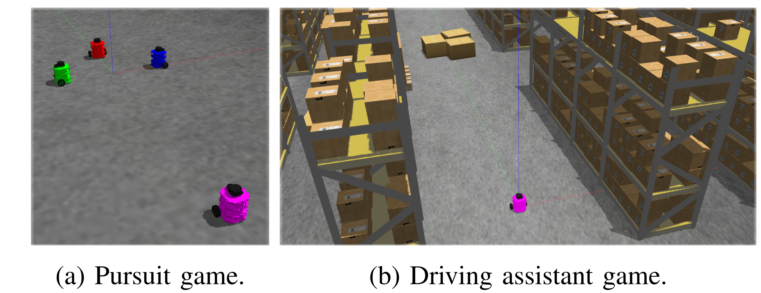
Two repeated games each have three hypotheses: identifying which of three leader-controlled rovers is pursued, and identifying a simulated follower’s response to a driving assistant. Julia, JuMP, and MOSEK solve the optimizations; splines transmit trajectories through ROS to virtual TurtleBots in Gazebo. Proportional controllers track them under tuned speed and maneuverability limits. No physical deployment or solver-time study is reported.
IV-A Leader-follower pursuit game parameters
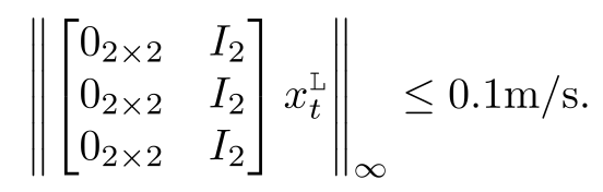
The pursuit setup uses planar double integrators and two-second discretization. The three follower types share tracking weights diag(20,20,0,0), input weight 30,000 times identity, and process covariance 10⁻⁵ times identity; their mappings select different leader rovers. Leader acceleration inputs are bounded by 0.005 and velocities by 0.1 m/s. The regularizer penalizes consecutive control differences. Identifying the type mainly requires separating candidate target trajectories.
Equation
IV-B Driving assistant game parameters
The driving task also uses two-second double-integrator dynamics, with follower process covariance 10⁻⁴ and leader covariance 10⁻⁷ times identity. Three mappings scale state/velocity reference components down, leave them unchanged, or scale them up; cost weights are shared. Leader input bounds are 0.05. A sideways L-shaped road has width 1.3 m and short-segment length 3 m; road and non-reversal constraints reduce feasible excitation. These are stylized simulated driver types, not empirically validated human categories.
IV-C Experimental procedure
At each two-second update the leader observes both states, optimizes a finite-horizon input sequence, shares its simulated trajectory, and executes the first input. The follower solves its maximum-entropy tracking problem for that reference, samples the first Gaussian action, and executes it. Both replan. This assumes state observation and communication of the planned leader trajectory, rather than inference from noisy partial visual observations alone.
IV-D Results
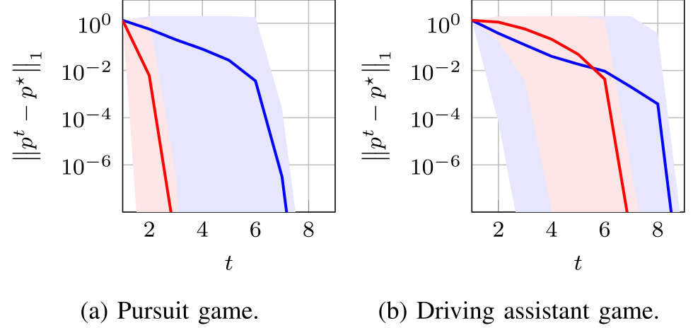
With a uniform prior and the first hypothesis as ground truth, evaluation measures the ℓ₁ distance between the posterior and the correct one-hot distribution. Figure 2 reports medians and first/third quartiles over one hundred simulations. The baseline samples allowed state trajectories uniformly and projects them through feasible tracking optimization; it is not uncontrolled random action noise.
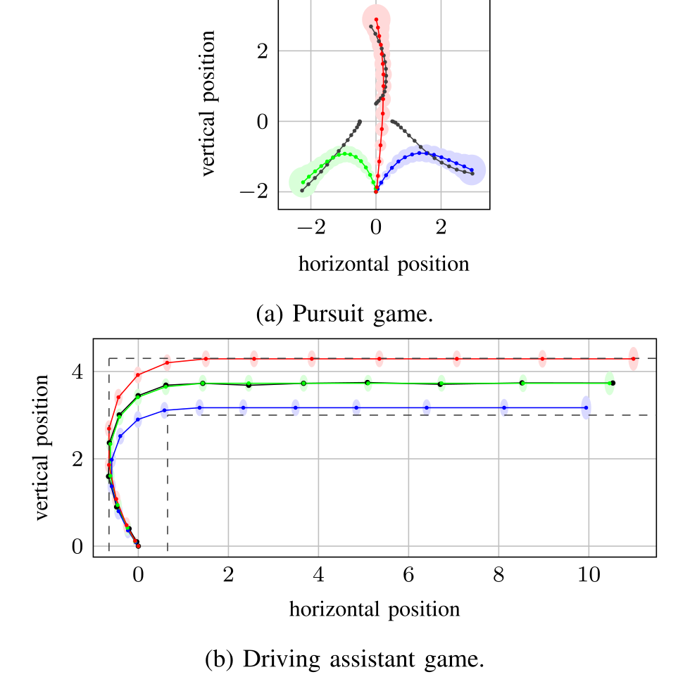
Active planning spreads pursuit targets in different directions and gives orders-of-magnitude smaller posterior error in the shown horizon. Driving gains become clear only after about six seconds, with less excitation available under road constraints. Figures 1 and 3 show responses and virtual-warehouse execution. Alternative information-gain planners, real humans, and collision safety are not evaluated. The authors provide a simulation video, optimization code, and ROS simulation code.
Equation 18
(18)
Fig. 1: The trajectories of the leader (black) and followers under different hypotheses. Each color indicates one of the hypotheses. The semi-axis of the shaded ellipses represents the directions of the eigenvectors of the corresponding covariance matrices. Fig. 2: Comparing the convergence of when using the proposed method (red) versus sampling a random trajectory (blue). The solid lines show the median over 100 simulations, while the boundaries of the colored areas mark the corresponding first and third quartiles.Fig. 3: Simulating the results on TurtleBots in a virtual warehouse environment in Gazebo.
V Conclusion
Finite-model, linear-quadratic excitation improves identification in these two games. The authors leave nonlinear dynamics, collision avoidance, and deceptive followers unresolved, and propose broader Bayesian-game information gathering as future work. The method also depends on known candidate objectives and noise models; faster concentration in this synthetic setting does not establish calibrated inference under model mismatch.
APPENDIX
The appendix derives the follower’s optimal Gaussian policy and state-moment recursions. It supports the closed-form model, rather than proving global optimality of the difference-of-convex planner.
Proof of Proposition Proposition 1 .
Dynamic programming preserves a quadratic value function. Expected quadratic control and future-value costs introduce covariance trace terms; differentiation with respect to the Gaussian mean and covariance gives the feedback law and backward recursions. Gaussian propagation gives forward state moments using the standard joint Gaussian construction. The published derivation and final unnumbered block are retained. Some appendix indices/covariance terms appear inconsistent with surrounding definitions; they remain visible as published rather than being rewritten into an unverified corrected proof.
Equations 19–23
(19)
(20)
(21)
(22)
(23)
ACKNOWLEDGMENT
The work acknowledges a National Science Foundation CAREER award and three additional NSF grants, plus Office of Naval Research subcontracts with Phillips and the University of Pennsylvania.
47 references
[1]V. A. Shia, Y. Gao, R. Vasudevan, K. D. Campbell, T. Lin, F. Borrelli, and
R. Bajcsy, “Semiautonomous vehicular control using driver modeling,”
IEEE Trans. Intel. Transp. Syst., vol. 15, no. 6, pp. 2696–2709,
2014.
[2]N. Mehr, R. Horowitz, and A. D. Dragan, “Inferring and assisting with
constraints in shared autonomy,” in Pro. IEEE Conf. Decision
Control. IEEE, 2016, pp. 6689–6696.
[4]D. Sadigh, S. S. Sastry, S. A. Seshia, and A. Dragan, “Information gathering
actions over human internal state,” in Proc. Int. Conf. Intel. Robots
Syst.IEEE, 2016, pp. 66–73.
[6]V. Kuleshov and O. Schrijvers, “Inverse game theory: Learning utilities in
succinct games,” in Int. Conf. Web Internet Econ. Springer, 2015, pp. 413–427.
[7]D. Bertsimas, V. Gupta, and I. C. Paschalidis, “Data-driven estimation in
equilibrium using inverse optimization,” Math. Prog., vol. 153,
no. 2, pp. 595–633, 2015.
[8]L. Peters, D. Fridovich-Keil, V. R. Royo, C. J. Tomlin, and C. Stachniss,
“Inferring objectives in continuous dynamic games from noise-corrupted
partial state observations,” in Robotics: Sci. and Syst. 2021, 2021.
[10]Y. Yu, J. Salfity, D. Fridovich-Keil, and U. Topcu, “Inverse matrix games with
unique quantal response equilibrium,” IEEE Control Syst. Lett.,
vol. 7, pp. 643–648, 2022.
[11]J. Li, C.-Y. Chiu, L. Peters, S. Sojoudi, C. Tomlin, and D. Fridovich-Keil,
“Cost inference for feedback dynamic games from noisy partial state
observations and incomplete trajectories,” in Proc. Int. Conf. Auton.
Agents and Multiagent Syst., 2023, pp. 1062–1070.
[12]C. K. Ling, F. Fang, and J. Z. Kolter, “What game are we playing? end-to-end
learning in normal and extensive form games,” in Proc. Int. Joint
Conf. Artif. Intell., 2018, pp. 396–402.
[13]S. Chen, Y. Yu, D. Fridovich-Keil, and U. Topcu, “Soft-bellman equilibrium in
affine markov games: Forward solutions and inverse learning,” arXiv
preprint arXiv:2304.00163, 2023.
[16]M. Lopes, F. Melo, and L. Montesano, “Active learning for reward estimation in
inverse reinforcement learning,” in Proc. Eur. Conf. Mach. Learn.
Knowl. Discovery Databases. Springer
Berlin Heidelberg, 2009, pp. 31–46.
[17]R. Akrour, M. Schoenauer, and M. Sebag, “April: Active preference
learning-based reinforcement learning,” in Proc. Eur. Conf. Mach.
Learn. Knowl. Discovery Databases. Springer, 2012, pp. 116–131.
[18]D. Sadigh, A. Dragan, S. Sastry, and S. Seshia, “Active preference-based
learning of reward functions,” in Robotics: Science and Systems
XIII, July 2017.
[19]P. F. Christiano, J. Leike, T. Brown, M. Martic, S. Legg, and D. Amodei, “Deep
reinforcement learning from human preferences,” Adv. Neural Inform.
Process. Syst., vol. 30, 2017.
[22]E. Bıyık, D. A. Lazar, D. Sadigh, and R. Pedarsani, “The green choice:
Learning and influencing human decisions on shared roads,” in Proc.
IEEE Conf. Decision Control. IEEE,
2019, pp. 347–354.
[23]M. Palan, G. Shevchuk, N. Charles Landolfi, and D. Sadigh, “Learning reward
functions by integrating human demonstrations and preferences,” in
Robot.: Sci. Syst., 2019.
[24]S. M. Katz, A.-C. Le Bihan, and M. J. Kochenderfer, “Learning an urban air
mobility encounter model from expert preferences,” in Proc. IEEE/AIAA
Digit. Avionics Syst. Conf.IEEE,
2019, pp. 1–8.
[25]C. Basu, E. Bıyık, Z. He, M. Singhal, and D. Sadigh, “Active learning of
reward dynamics from hierarchical queries,” in Proc. IEEE/RSJ Int.
Conf. Intell. Robots Syst.IEEE,
2019, pp. 120–127.
[26]R. Cohn, E. Durfee, and S. Singh, “Comparing action-query strategies in
semi-autonomous agents,” in Proc. AAAI Conf. on Artif. Intell.,
vol. 25, no. 1, 2011, pp. 1102–1107.
[27]C. Daniel, O. Kroemer, M. Viering, J. Metz, and J. Peters, “Active reward
learning with a novel acquisition function,” Autonomous Robots,
vol. 39, pp. 389–405, 2015.
[29]E. Bıyık, M. Palan, N. C. Landolfi, D. P. Losey, and D. Sadigh, “Asking
easy questions: A user-friendly approach to active reward learning,” in
Conf. Robot Learn.PMLR, 2020,
pp. 1177–1190.
[35]B. D. Ziebart, A. L. Maas, J. A. Bagnell, and A. Dey, “Maximum entropy inverse
reinforcement learning.” in Proc. AAAI Conf. on Artif. Intell.,
vol. 3, 2008, pp. 1433–1438.
[37]Z. Wu, L. Sun, W. Zhan, C. Yang, and M. Tomizuka, “Efficient sampling-based
maximum entropy inverse reinforcement learning with application to autonomous
driving,” IEEE Robot. Automat. Lett., vol. 5, no. 4, pp. 5355–5362,
2020.
[40]J. Bezanson, A. Edelman, S. Karpinski, and V. B. Shah, “Julia: A fresh
approach to numerical computing,” SIAM review, vol. 59, no. 1, pp.
65–98, 2017. [Online]. Available: https://doi.org/10.1137/141000671
[41]M. Lubin, O. Dowson, J. Dias Garcia, J. Huchette, B. Legat, and J. P. Vielma,
“JuMP 1.0: Recent improvements to a modeling language for mathematical
optimization,” Math. Program. Comput., 2023.
[46]T. Fischer, W. Vollprecht, S. Traversaro, S. Yen, C. Herrero, and M. Milford,
“A robostack tutorial: Using the robot operating system alongside the conda
and jupyter data science ecosystems,” IEEE Robot. Automat. Mag.,
2021.