The full paper and both appendices are condensed below. Original figures, captions, displayed definitions and derivations, references, and author portraits are preserved.
Maulik Bhatt is a Ph.D. student in the Department of Mechanical Engineering at UC Berkeley. Before joining Berkeley, he was a Ph.D. student in the Department of Aerospace Engineering at the University of Illinois Urbana-Champaign. He received his Interdisciplinary Dual Degree (Bachelor’s in Aerospace Engineering + Master’s in Systems and Control Engineering) from the Indian Institute of Technology Bombay in 2021. He is interested in leveraging game theory, stochastic control, and machine learning to enable efficient robotic multi-agent interactions and safe motion planning. During his undergraduate studies, he worked in the area of state estimation using geometric control and variational principles.
Yixuan Jia received B.S. degrees in computer engineering and mathematics from the University of Illinois Urbana-Champaign, Champaign, IL, USA, in 2023. During his undergraduate studies, he studied multi-agent planning, safety verification of autonomous systems, and control theory.
He is currently working toward the M.S. degree in Aeronautics and Astronautics at the Massachusetts Institute of Technology.
His current research interests include perception, localization, and planning for autonomous navigation in unstructured environments.
Negar Mehr (Member, IEEE) received a B.S. degree from the Sharif University of Technology and a Ph.D. degree from UC Berkeley, Berkeley, CA, USA, in 2013 and 2019, respectively, both in mechanical engineering. From 2019 to 2020, she was a Postdoctoral Scholar with Stanford Aeronautics and Astronautics Department. She is an Assistant Professor with the Mechanical Engineering Department at the University of California. Berkeley. Before joining Berkeley, she was an assistant professor in Aerospace Engineering at the University of Illinois Urbana-Champaign. Her research interest includes learning and control algorithms for interactive robots, robots that can safely and intelligently interact with other agents. Dr. Mehr is the recipient of the NSFCAREER award in 2022. Her Ph.D. dissertation was awarded the 2020 IEEEITSS Best Ph.D. Dissertation Award.
At a glance
The paper identifies structured multi-agent planning problems whose individual objectives can be represented through a weighted potential. It then replaces several coupled optimal-control problems with one constrained trajectory optimization. Shared pairwise cost shapes can still have asymmetric importance weights. Simulations show lower solve times on the tested problems, and two quadrotors carry a rigid rod around two people in a laboratory demonstration. The reduction applies to specified cost structures and information assumptions, not arbitrary strategic interactions.
I Introduction
Game-theoretic planning accounts for how other agents may react, but directly solving coupled nonlinear trajectory problems is expensive. The proposed simplification uses potential-game structure [3] when agents share space or tasks. Earlier exact-potential formulations emphasized symmetric interactions; this work allows particular asymmetries through positive weights. Its contributions are explicit cost constructions for two or more agents, a potential-based optimal-control formulation, numerical comparisons, and a constrained aerial-transport demonstration. Speed gains arise from exploiting this structure rather than solving unrestricted games faster.
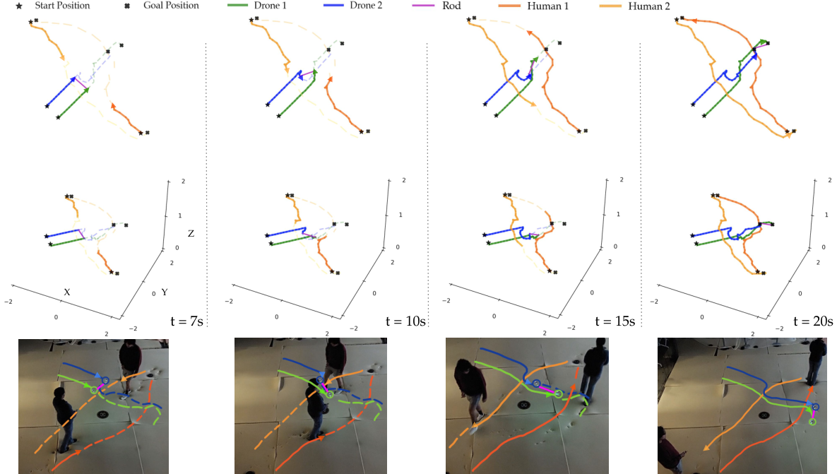
Fig. 1: Visualizations and the corresponding snapshots of the hardware experiment.
The two quadrotors and two humans need to reach their designated goal positions while avoiding collision with others. The two quadrotors are carrying a rod. In this case, each quadrotor needs to account for the motions of humans as well as the other quadrotor, as they share the constraint imposed by the rod.
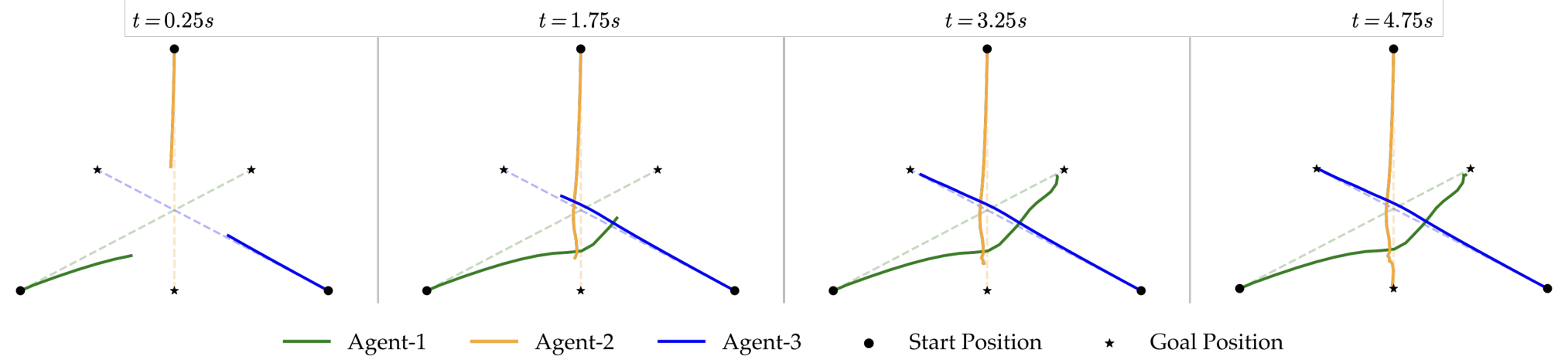
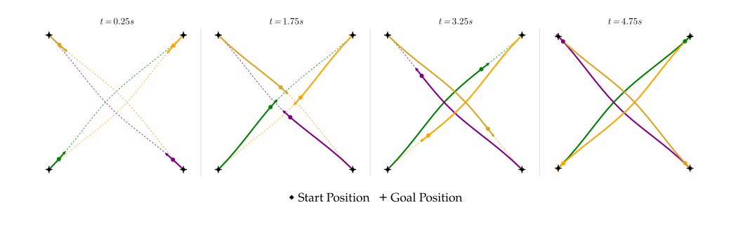
As shown in the figure, with our algorithm, the two quadrotors are able to avoid nearby humans by changing their orientations elegantly while carrying the rod. (Refer to Appendix -B for the approval details for conducting experiments with human subjects.) We have also included a supplementary video of the experiment which will be available at http://ieeexplore.ieee.org.Fig. 2: The snapshots of the trajectories found by our algorithm when three unicycle agents interact with each other and exchange their positions diagonally over a time interval of 5s. The cost functions are highly asymmetric, and Agent 1 incurs more costs for getting close to other agents. Agents move from their start positions to their respective goal positions. Dashed lines represent the nominal path for each agent. Because of the asymmetric nature of the interaction, Agent 1 yields to other agents and deviates more from its nominal path to move towards its goal.
II Related Work
II-A Multi-agent Motion Planning
Cooperative planners and learned navigation policies address related coordination problems. The paper focuses on agents with individual objectives and shared feasibility constraints, where predicting reactions is part of planning. Its criticism of prior methods is a motivation for the chosen game model, not evidence that all learning-based or cooperative methods lack interaction reasoning.
II-B Game-Theoretic Multi-Agent Interactions
Prior game solvers use leader–follower models, sampled trajectories, iterated best responses, local quadratic approximations, augmented Lagrangians, or stochastic and belief-space formulations. Repeatedly solving coupled nonconvex responses can be expensive. The proposed method trades that generality for a class where one potential objective captures the relevant individual incentives.
II-C Potential Games
Static, differential, and discrete-time potential games appear in resource allocation and control. This paper extends potential-based robot planning beyond equal pairwise cost coefficients while retaining shared pairwise functional forms.
III Notation and Preliminaries
Each agent has its own state and control, with dynamics depending only on its own variables. Agents interact through costs and shared state/control constraints; a rigid-object relation is represented as a constraint rather than coupled dynamics. Costs sum stage and terminal terms and depend on all states but only the agent’s own controls. Feasible strategies satisfy dynamics and constraints throughout the horizon. An open-loop generalized Nash equilibrium is a feasible collection of complete trajectories for which no agent can reduce its cost through a feasible unilateral change. The information model assumes known initial state, other agents’ dynamics, and their objectives. Repeated open-loop optimization is used in a receding horizon to react to new measurements. This can approximate feedback behavior but is not generally the same as a feedback Nash equilibrium.
Equations 1–6
(1)
(2)
(3)
(4)
(5)
(6)
IV Constrained Potential Dynamic Games
An exact potential reproduces the total cost change caused by any unilateral strategy change. The paper’s weighted definition introduces positive agent- and stage-dependent factors. Lemmas 1 and 2 characterize the proposed structure through proportional own-state/own-control derivatives, or an equivalent stage-cost decomposition into a scaled common term plus a remainder independent of that agent’s variables. Separable dynamics keep other agents’ trajectories fixed during a unilateral open-loop deviation. Costs, dynamics, and constraints are assumed differentiable, with constraint regularity. Theorem 1 states that solving the resulting constrained potential-minimization problem yields an open-loop generalized equilibrium. The appendix argues through first-order optimality conditions; this should not be read as a general guarantee that a local nonconvex solver returns a global equilibrium. Each agent may independently solve a copy, but multiple equilibria can cause incompatible selections; alignment of those choices is left outside the method.
Equations 7–17
(7)
(8)
(9)
(10)
(11)
(12)
(13)
(14)
(15)
(16)
subject to
(17)
V Dyadic Interactions
For two agents, each stage cost combines an individual term and a positively weighted shared interaction function. The interaction shapes must match when the agents are exchanged, although their coefficients may differ. The proposed potential scales agent 1’s individual term by agent 2’s coefficient, agent 2’s individual term by agent 1’s coefficient, and the shared interaction term by the coefficient product. Lemma 3 uses reciprocal opposite-agent coefficients as weights. This covers asymmetric aversion to proximity when both agents use the same distance-based cost shape. It does not show that every two-player game is a potential game. The displayed derivation is retained, including the source’s inconsistent repeated denominator for agent 2 in the explanatory proof text; the lemma statement and potential construction specify the intended opposite-agent scaling.
Equations 18a–25
(18a)
(18b)
(19a)
(19b)
(20)
(21)
(22)
(23)
(24)
(25)
VI Multi-agent Interactions
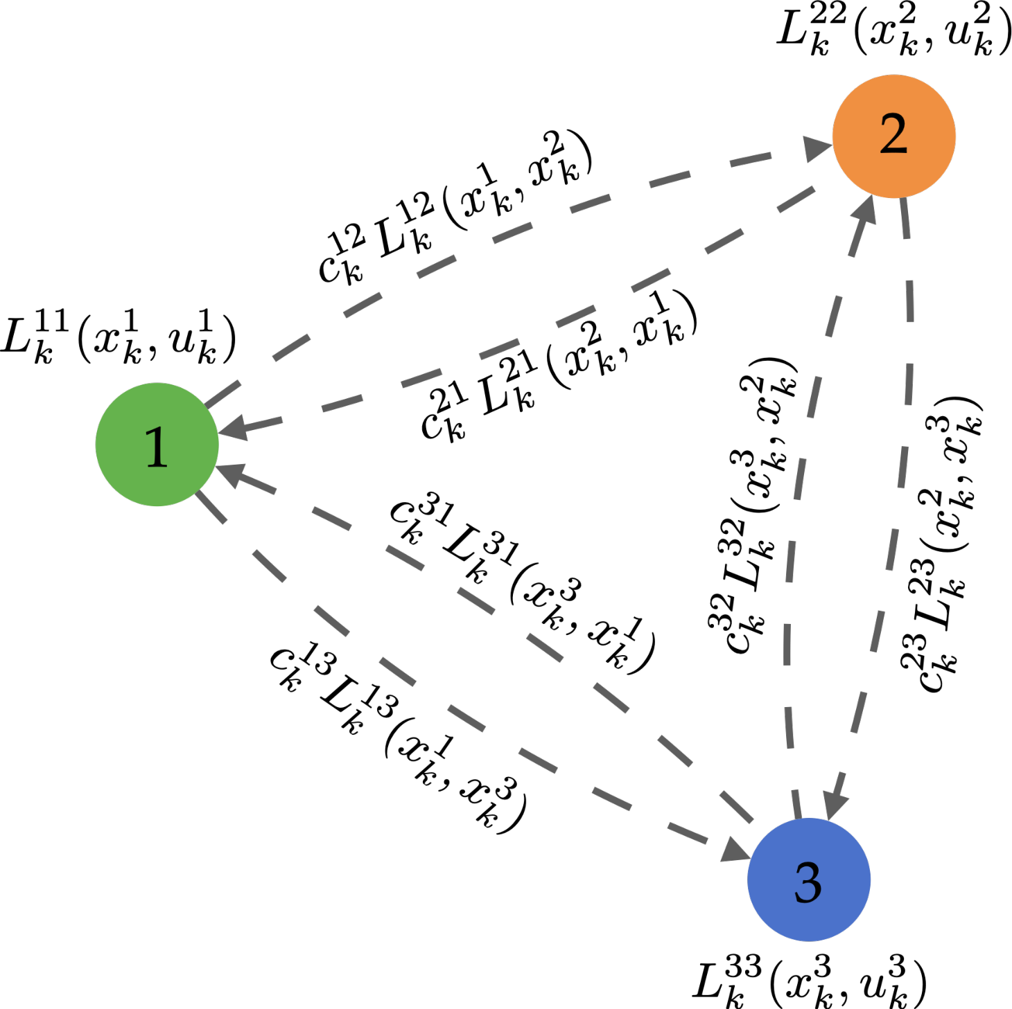
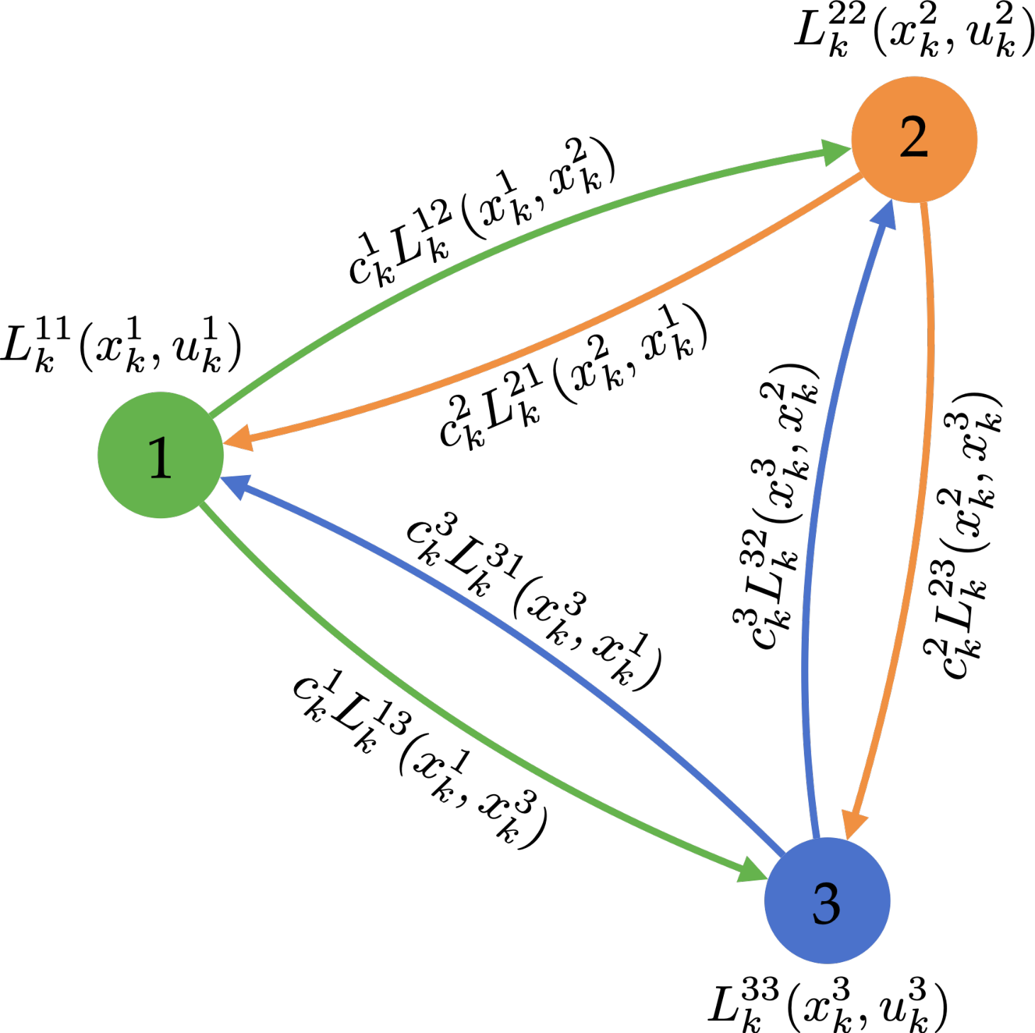
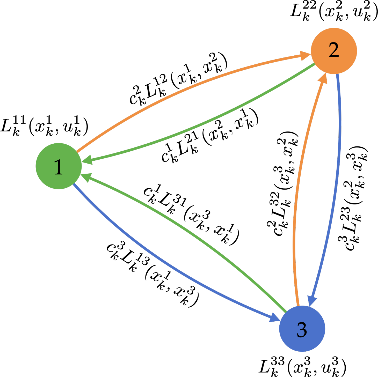
For more agents, costs combine individual terms with symmetric-shape pairwise interactions and positive directed coefficients. Two sufficient coefficient patterns are developed. In the first, an agent gives every other agent the same coefficient, although different agents may be more or less cautious. In the second, every agent assigns a given counterpart the same coefficient, so the counterpart’s identity determines its weight. The figures distinguish these outgoing- and incoming-coefficient patterns. The corresponding potentials sum reweighted individual terms and each unordered pair once; the proofs separate terms that cannot change under the selected agent’s unilateral deviation. Noninteracting pairs may have zero interaction functions. These constructions do not cover arbitrary directed coefficient matrices or different pairwise cost shapes. Unconstrained examples use iterative LQR; constrained examples use ALTRO, which combines an augmented Lagrangian, iterative LQR, and active-set refinement.
Equations 26a–26b
(26a)
and
(26b)
Fig. 3: Schematic of the cost function dependencies for a running example with three agents interacting with one another.Equations 27–29
(27)
(28)
(29)
Fig. 4: Schematic of an interaction where each agent in the environment treats all the other agents in a similar fashion. In such scenarios, the underlying dynamic game becomes a weighted potential dynamic game. Note that in this figure, the edges with the same color indicate the same value of the cost coefficient.Equations 30–32
(30)
(31)
(32)
Fig. 5: Schematic of interactions where each agent in the environment is treated by all the other agents in a similar fashion. In such scenarios, the underlying dynamic game becomes a weighted potential dynamic game. It should be noted that edges with the same color indicate the same value of the cost coefficient.Equations 33–37
(33)
(34)
(35)
(36)
(37)
VII Simulations Studies
Experiments first check a linear-quadratic case with an analytic equilibrium, then test nonlinear navigation and runtime.
VII-A Dyadic Linear Quadratic Interactions
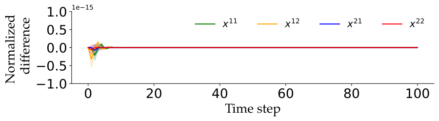
A two-player linear-quadratic example specifies complete dynamics and cost matrices. An equivalent exact-potential problem is solved through the ordinary discrete-time LQR Riccati equations and compared with the analytic open-loop game solution. Across 200 nearby random initial states, trajectory differences are at numerical precision. This is a useful check of that particular structured case; it does not validate every nonlinear or time-varying weighted case. The original matrix displays, including their labels, remain unchanged.
Equations 38–40
(38)
(39)
(40)
Fig. 6: Comparison of trajectories for the LQ-game solved using potential minimization and exact open-loop Nash solution shows that the trajectories generated are close up to the system precision level.Equations 41–44
(41)
(42)
(43)
(44)
Fig. 7: The snapshots of the trajectories found by our algorithm when four unicycle agents interact with each other and exchange their positions diagonally over a time interval of 5s. Agents move from their start positions to their respective goal positions. In order to avoid collision with other agents, each agent deviates from its nominal trajectory and successfully reaches its goal position.
VII-B Multi-agent Interactive Planning
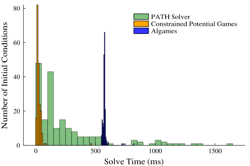
Three unicycle agents exchange positions with a soft proximity penalty inside 2 m. Assigning agent 1 a larger penalty makes it deviate more, illustrating modeled asymmetry. A separate four-agent example starts at the corners of a 3 m square, sends agents toward opposite corners, and imposes a 0.3 m minimum separation plus control bounds. The source describes the second control as acceleration in its dynamics but later describes a bound in linear-velocity units, an implementation detail that requires clarification when reproducing the setup. Runtime comparisons use 200 random initial conditions and matched initializations: the potential method averages 26.15±34.30 ms, ALGAMES 577.35±27.70 ms, and PATH 248.21±302.05 ms. PATH converges in 189/200 runs, and its reported time excludes failures. Thus the roughly tenfold and twentyfold mean speedups are specific to this four-agent benchmark and its convergence accounting.
Equations 45–49
(45)
(46)
(47)
(48)
(49)
Fig. 8: Histograms for the comparison of the solve time of Constrained Potential Games with Algames. Constrained Potential Games has an average solve time of 26.15 ms in contrast to the PATH solver and Algames, which have an average solve time of 248.21 and 577.35 ms, respectively. Our approach is approximately 10 times faster than the PATH solver and 20 times faster than Algames.
VIII Experiments
Two Crazyflie quadrotors carry a 0.5 m rigid rod while two people walk toward designated goals. The planner enforces fixed inter-quadrotor separation and collision constraints. Quadrotors are modeled as six-degree-of-freedom integrators because existing Crazyswarm low-level controllers track supplied waypoints; this is not full coupled aerial-load dynamics. People use unicycle models and 2 m-high, 0.4 m-radius collision cylinders. Human goals are supplied and their objectives are assumed to resemble straight-line goal tracking with effort penalties. Maximum linear speeds are 1.2 m/s for drones and 1.5 m/s for people. A 0.5 s horizon with 0.1 s steps is solved using do-mpc, CasADi, and IPOPT. Replanning partly handles prediction mismatch, but the authors explicitly note that substantially different human costs can cause poor behavior. Figure 1 demonstrates coordinated rod rotation and avoidance in this setup; the paper does not report a broad human-behavior or safety evaluation.
Equations
IX Conclusion
Potential structure can make the tested strategic planning problems much cheaper to optimize. The price is restricted interaction costs, known or estimated objectives, separable modeled dynamics, and unresolved equilibrium-selection issues. Future work proposes more general cost shapes and learned objectives. The current demonstrations should be distinguished from guarantees for unfamiliar human behavior, arbitrary games, or global convergence of nonconvex optimization.
-A Proof of Theorem 1
The appendix writes agent-wise and potential-problem Lagrangians, then compares their stationarity, primal feasibility, dual feasibility, and complementarity conditions using derivative proportionality and multiplier rescaling. Regularity is invoked to justify necessary optimality conditions. Reader qualification: matching such conditions does not by itself establish global best-response optimality in a nonconvex problem. Stage-dependent weights also require care across the costate recurrence: rescaling neighboring-time multipliers independently is not automatically equivalent to one fixed positive scaling of the total trajectory objective. The original derivation and all formulas are preserved for inspection rather than silently repaired.
Equations 50–74
(50)
(51)
(52)
(53)
(54)
(55)
(56)
(57)
(58)
(59)
(60)
(61)
(62)
(63)
(64)
(65)
(66)
(67)
(68)
(69)
(70)
(71)
(72)
(73)
(74)
-B Exempt Determination Involving Human Subjects
The authors report that the University of Illinois Urbana-Champaign Office for the Protection of Research Subjects determined the human-subject experiment exempt under protocol 22107.
55 references
[1]
T. Başar and G. J. Olsder, Dynamic noncooperative game theory. SIAM, 1998.
[2]
R. Isaacs, Differential games: a mathematical theory with applications to warfare and pursuit, control and optimization. Courier Corporation, 1999.
[4]
T. Kavuncu, A. Yaraneri, and N. Mehr, “Potential ilqr: A potential-minimizing controller for planning multi-agent interactive trajectories,” arXiv preprint arXiv:2107.04926, 2021.
[5]
M. Bhatt, A. Yaraneri, and N. Mehr, “Efficient constrained multi-agent interactive planning using constrained dynamic potential games,” arXiv preprint arXiv:2206.08963, 2022.
[6]
T. A. Howell, B. E. Jackson, and Z. Manchester, “Altro: A fast solver for constrained trajectory optimization,” in 2019 IEEE/RSJ International Conference on Intelligent Robots and Systems (IROS). IEEE, 2019, pp. 7674–7679.
[7]
S. Lucia, A. Tătulea-Codrean, C. Schoppmeyer, and S. Engell, “Rapid development of modular and sustainable nonlinear model predictive control solutions,” Control Engineering Practice, vol. 60, pp. 51–62, 2017.
[8]
W. Li and E. Todorov, “Iterative linear quadratic regulator design for nonlinear biological movement systems,” in First International Conference on Informatics in Control, Automation and Robotics, vol. 2. SciTePress, 2004, pp. 222–229.
[9]
J. Yu and S. M. LaValle, “Optimal multirobot path planning on graphs: Complete algorithms and effective heuristics,” IEEE Transactions on Robotics, vol. 32, no. 5, pp. 1163–1177, 2016.
[10]
S. Tang, J. Thomas, and V. Kumar, “Hold or take optimal plan (hoop): A quadratic programming approach to multi-robot trajectory generation,” The International Journal of Robotics Research, vol. 37, no. 9, pp. 1062–1084, 2018.
[11]
F. Augugliaro, A. P. Schoellig, and R. D’Andrea, “Generation of collision-free trajectories for a quadrocopter fleet: A sequential convex programming approach,” in 2012 IEEE/RSJ international conference on Intelligent Robots and Systems. IEEE, 2012, pp. 1917–1922.
[12]
V. R. Desaraju and J. P. How, “Decentralized path planning for multi-agent teams with complex constraints,” Autonomous Robots, vol. 32, pp. 385–403, 2012.
[13]
C. Toumieh and A. Lambert, “Decentralized multi-agent planning using model predictive control and time-aware safe corridors,” IEEE Robotics and Automation Letters, vol. 7, no. 4, pp. 11 110–11 117, 2022.
[14]
D. Zhou, Z. Wang, S. Bandyopadhyay, and M. Schwager, “Fast, on-line collision avoidance for dynamic vehicles using buffered voronoi cells,” IEEE Robotics and Automation Letters, vol. 2, no. 2, pp. 1047–1054, 2017.
[16]
H. Qie, D. Shi, T. Shen, X. Xu, Y. Li, and L. Wang, “Joint optimization of multi-uav target assignment and path planning based on multi-agent reinforcement learning,” IEEE access, vol. 7, pp. 146 264–146 272, 2019.
[17]
Z. Liu, B. Chen, H. Zhou, G. Koushik, M. Hebert, and D. Zhao, “Mapper: Multi-agent path planning with evolutionary reinforcement learning in mixed dynamic environments,” in 2020 IEEE/RSJ International Conference on Intelligent Robots and Systems (IROS). IEEE, 2020, pp. 11 748–11 754.
[18]
S. H. Semnani, H. Liu, M. Everett, A. De Ruiter, and J. P. How, “Multi-agent motion planning for dense and dynamic environments via deep reinforcement learning,” IEEE Robotics and Automation Letters, vol. 5, no. 2, pp. 3221–3226, 2020.
[19]
A. P. Vinod, S. Safaoui, A. Chakrabarty, R. Quirynen, N. Yoshikawa, and S. Di Cairano, “Safe multi-agent motion planning via filtered reinforcement learning,” in 2022 International Conference on Robotics and Automation (ICRA). IEEE, 2022, pp. 7270–7276.
[20]
G. Papoudakis, F. Christianos, A. Rahman, and S. V. Albrecht, “Dealing with non-stationarity in multi-agent deep reinforcement learning,” arXiv preprint arXiv:1906.04737, 2019.
[21]
C. S. De Witt, T. Gupta, D. Makoviichuk, V. Makoviychuk, P. H. Torr, M. Sun, and S. Whiteson, “Is independent learning all you need in the starcraft multi-agent challenge?” arXiv preprint arXiv:2011.09533, 2020.
[22]
H. Kretzschmar, M. Spies, C. Sprunk, and W. Burgard, “Socially compliant mobile robot navigation via inverse reinforcement learning,” The International Journal of Robotics Research, vol. 35, no. 11, pp. 1289–1307, 2016.
[23]
S. Parsons and M. Wooldridge, “Game theory and decision theory in multi-agent systems,” Autonomous Agents and Multi-Agent Systems, vol. 5, pp. 243–254, 2002.
[24]
D. Sadigh, S. Sastry, S. A. Seshia, and A. D. Dragan, “Planning for autonomous cars that leverage effects on human actions.” in Robotics: Science and systems, vol. 2. Ann Arbor, MI, USA, 2016, pp. 1–9.
[25]
J. F. Fisac, E. Bronstein, E. Stefansson, D. Sadigh, S. S. Sastry, and A. D. Dragan, “Hierarchical game-theoretic planning for autonomous vehicles,” in 2019 International conference on robotics and automation (ICRA). IEEE, 2019, pp. 9590–9596.
[26]
A. Turnwald and D. Wollherr, “Human-like motion planning based on game theoretic decision making,” International Journal of Social Robotics, vol. 11, pp. 151–170, 2019.
[27]
R. Spica, E. Cristofalo, Z. Wang, E. Montijano, and M. Schwager, “A real-time game theoretic planner for autonomous two-player drone racing,” IEEE Transactions on Robotics, vol. 36, no. 5, pp. 1389–1403, 2020.
[28]
M. Wang, Z. Wang, J. Talbot, J. C. Gerdes, and M. Schwager, “Game theoretic planning for self-driving cars in competitive scenarios.” in Robotics: Science and Systems, 2019.
[29]
Z. Wang, R. Spica, and M. Schwager, “Game theoretic motion planning for multi-robot racing,” in Distributed Autonomous Robotic Systems: The 14th International Symposium. Springer, 2019, pp. 225–238.
[30]
K. Miller and S. Mitra, “Multi-agent motion planning using differential games with lexicographic preferences,” in 2022 IEEE 61st Conference on Decision and Control (CDC). IEEE, 2022, pp. 5751–5756.
[31]
D. Fridovich-Keil, E. Ratner, L. Peters, A. D. Dragan, and C. J. Tomlin, “Efficient iterative linear-quadratic approximations for nonlinear multi-player general-sum differential games,” in 2020 IEEE international conference on robotics and automation (ICRA). IEEE, 2020, pp. 1475–1481.
[32]
W. Schwarting, A. Pierson, S. Karaman, and D. Rus, “Stochastic dynamic games in belief space,” IEEE Transactions on Robotics, vol. 37, no. 6, pp. 2157–2172, 2021.
[33]
S. Le Cleac’h, M. Schwager, and Z. Manchester, “Algames: a fast augmented lagrangian solver for constrained dynamic games,” Autonomous Robots, vol. 46, no. 1, pp. 201–215, 2022.
[34]
F. Laine, D. Fridovich-Keil, C.-Y. Chiu, and C. Tomlin, “The computation of approximate generalized feedback nash equilibria,” SIAM Journal on Optimization, vol. 33, no. 1, pp. 294–318, 2023.
[35]
M. Wang, N. Mehr, A. Gaidon, and M. Schwager, “Game-theoretic planning for risk-aware interactive agents,” in 2020 IEEE/RSJ International Conference on Intelligent Robots and Systems (IROS). IEEE, 2020, pp. 6998–7005.
[36]
N. Mehr, M. Wang, M. Bhatt, and M. Schwager, “Maximum-entropy multi-agent dynamic games: Forward and inverse solutions,” IEEE Transactions on Robotics, 2023.
[37]
M. Chahine, R. Firoozi, W. Xiao, M. Schwager, and D. Rus, “Intention communication and hypothesis likelihood in game-theoretic motion planning,” IEEE Robotics and Automation Letters, vol. 8, no. 3, pp. 1223–1230, 2023.
[38]
R. W. Rosenthal, “A class of games possessing pure-strategy nash equilibria,” International Journal of Game Theory, vol. 2, no. 1, pp. 65–67, 1973.
[40]
G. Arslan, J. R. Marden, and J. S. Shamma, “Autonomous Vehicle-Target Assignment: A Game-Theoretical Formulation,” Journal of Dynamic Systems, Measurement, and Control, vol. 129, no. 5, pp. 584–596, 04 2007. [Online]. Available: https://doi.org/10.1115/1.2766722
[41]
J. R. Marden, G. Arslan, and J. S. Shamma, “Cooperative control and potential games,” IEEE Transactions on Systems, Man, and Cybernetics, Part B (Cybernetics), vol. 39, no. 6, pp. 1393–1407, 2009.
[42]
S. Zazo, J. Zazo, and M. Sánchez-Fernández, “A control theoretic approach to solve a constrained uplink power dynamic game,” in 2014 22nd European Signal Processing Conference (EUSIPCO). IEEE, 2014, pp. 401–405.
[43]
S. Zazo, S. V. Macua, M. Sánchez-Fernández, and J. Zazo, “Dynamic potential games with constraints: Fundamentals and applications in communications,” IEEE Transactions on Signal Processing, vol. 64, no. 14, pp. 3806–3821, 2016.
[44]
Z. Williams, J. Chen, and N. Mehr, “Distributed potential ilqr: Scalable game-theoretic trajectory planning for multi-agent interactions,” arXiv preprint arXiv:2303.04842, 2023.
[45]
Y. Jia, M. Bhatt, and N. Mehr, “Rapid: Autonomous multi-agent racing using constrained potential dynamic games,” arXiv preprint arXiv:2305.00579, 2023.
[46]
J. Li, C.-Y. Chiu, L. Peters, S. Sojoudi, C. Tomlin, and D. Fridovich-Keil, “Cost inference for feedback dynamic games from noisy partial state observations and incomplete trajectories,” arXiv preprint arXiv:2301.01398, 2023.
[47]
L. Peters, D. Fridovich-Keil, C. J. Tomlin, and Z. N. Sunberg, “Inference-based strategy alignment for general-sum differential games,” arXiv preprint arXiv:2002.04354, 2020.
[49]
S. P. Dirkse and M. C. Ferris, “The path solver: a nommonotone stabilization scheme for mixed complementarity problems,” Optimization methods and software, vol. 5, no. 2, pp. 123–156, 1995.
[50]
X. Liu, L. Peters, and J. Alonso-Mora, “Learning to play trajectory games against opponents with unknown objectives,” IEEE Robotics and Automation Letters, 2023.
[52]
S. Russell, “Learning agents for uncertain environments,” in Proceedings of the eleventh annual conference on Computational learning theory, 1998, pp. 101–103.
[53]
J. A. E. Andersson, J. Gillis, G. Horn, J. B. Rawlings, and M. Diehl, “CasADi – A software framework for nonlinear optimization and optimal control,” Mathematical Programming Computation, vol. 11, no. 1, pp. 1–36, 2019.
[54]
A. Wächter and L. T. Biegler, “On the implementation of an interior-point filter line-search algorithm for large-scale nonlinear programming,” Mathematical Programming, vol. 106, no. 1, pp. 25–57, 2006.