Overview
At a glance
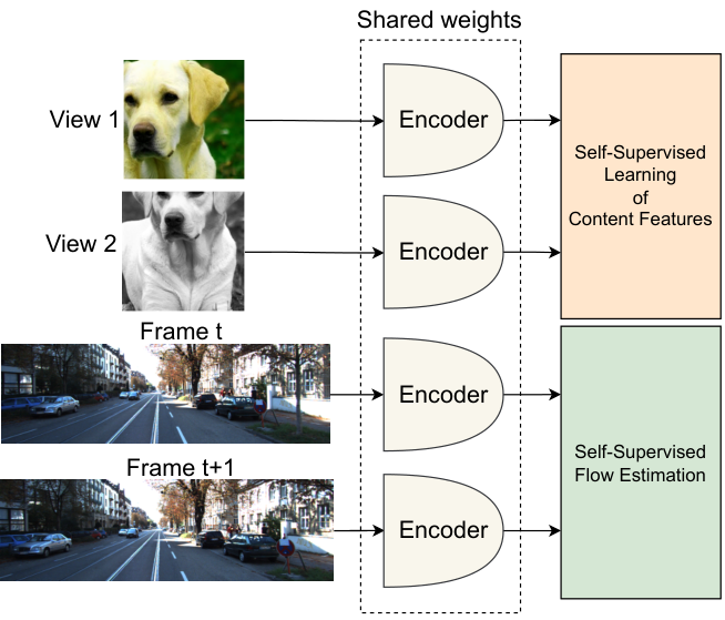
Recognizing a car and tracking which way it moves are related but different jobs. MC-JEPA trains one encoder to support both. One branch learns optical flow: how pixels correspond between successive frames. Another learns image content by making augmented views of the same image agree. Combining their training losses improves the shared features for motion and segmentation tasks. Unlike the later masked-feature-only V-JEPA recipe, this motion branch also uses photometric reconstruction and geometric consistency losses. The contribution is a tested multi-task representation-learning system, not a universal recipe for learning every aspect of a video or a planner for controlling actions.
1 Introduction
Most image self-supervision emphasizes semantic identity, while optical-flow systems emphasize precise correspondence. MC-JEPA connects them with shared encoder weights. Its motion-only component, M-JEPA, improves a coarse-to-fine flow estimator; combining it with VICReg image training yields MC-JEPA. Evaluation asks whether one encoder can support optical flow, image segmentation and video-object tracking rather than specializing entirely in one task.
2 Related Work
The related work separates global semantic learning, dense local learning, optical flow and video correspondence. Multi-task learning supplies the connection: motion supervision can improve localization, while semantic features can improve correspondence. The approach does not require that these objectives always agree; their relative weights and training stability are explicit engineering issues.
3 Proposed approach
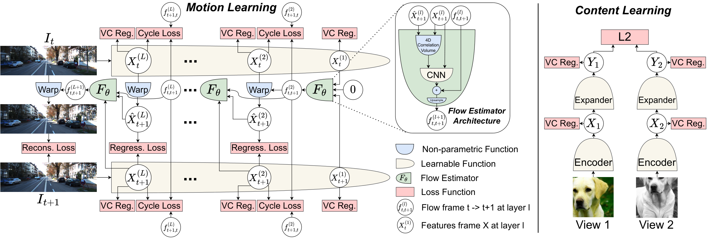
The method first builds a motion learner, then adds a semantic-learning branch. Both update the same encoder, while retaining their own prediction networks and losses.
3.1 Optical flow
Optical flow assigns a two-dimensional displacement to each pixel. A hierarchical estimator predicts coarse motion and refines it at progressively finer scales, using feature warping and correlations between frames. The losses check whether the predicted movement aligns features and reconstructs the corresponding image. Smoothness regularization helps where texture gives little evidence.
Forward–backward cycle consistency asks whether following predicted motion out and back returns to the original features. Occlusion handling excludes unreliable correspondences from the regression term. Variance–covariance penalties encourage informative, nonredundant encoder features. These pieces work together: low feature-prediction loss alone could otherwise be achieved with uninformative representations.
Equations 1–4
| (1) |
| (2) |
| (3) |
| (4) |
| Optical Flow Estimation | Image Segmentation | Video Seg. | |||||||||||||||||||
| Sintel Clean | Sintel Final | KITTI 2015 | Pascal VOC | CityScapes | ADE20k | Davis 2017 | |||||||||||||||
| Method | Backbone | train | test | train | test | train | test | Frozen | FT | Frozen | FT | Frozen | FT | ||||||||
| EPE | EPE | EPE | EPE | EPE | F1 | mIoU | mIoU | mIoU | mIoU | mIoU | mIoU | ||||||||||
| Rand. weights | CNX-T | 23.71 | - | 24.02 | - | 24.88 | - | 0.5 | - | - | - | - | - | - | |||||||
| flow methods | |||||||||||||||||||||
| UFlow (Jonschkowski et al., 2020) | PWC | 2.50 | 5.21 | 3.39 | 6.50 | 2.71 | 11.13 | 7.8 | - | - | - | - | - | 42.0 | |||||||
| ARFLow (Liu et al., 2020) | PWC | 2.79 | 4.78 | 3.73 | 5.89 | 2.85 | 11.80 | 7.9 | - | - | - | - | - | - | |||||||
| UPFlow (Luo et al., 2021) | PWC | 2.33 | 4.68 | 2.67 | 5.32 | 2.45 | 9.38 | 8.8 | - | - | - | - | - | - | |||||||
| SMURF (Stone et al., 2021) | RAFT | 1.71 | 3.15 | 2.58 | 4.18 | 2.00 | 6.83 | 10.4 | - | - | - | - | - | - | |||||||
| correspondence methods | |||||||||||||||||||||
| VFS (Xu & Wang, 2021) | R50 | - | - | - | - | - | - | 51.2 | - | - | - | - | - | 68.9 | |||||||
| MCRW (Bian et al., 2022) | PWC | 2.84 | 5.68 | 3.82 | 6.72 | 2.81 | 11.67 | 39.8 | - | - | - | - | - | 57.9 | |||||||
| content methods | |||||||||||||||||||||
| VICReg (Bardes et al., 2022a) | CNX-T | - | - | - | - | 13.5 | - | 60.1 | 77.8 | 59.8 | 76.3 | 28.6 | 41.1 | 58.1 | |||||||
| VICRegL (Bardes et al., 2022b) | CNX-T | - | - | - | - | 11.4 | - | 66.8 | 79.7 | 64.9 | 78.3 | 30.6 | 44.1 | 66.7 | |||||||
| MoCo v3 (Chen et al., 2021) | ViT-S | - | - | - | - | 12.9 | - | 57.1 | 75.9 | 56.5 | 74.0 | 23.7 | 39.8 | - | |||||||
| DINO (Caron et al., 2021) | ViT-S | - | - | - | - | 11.8 | - | 65.2 | 79.5 | 64.8 | 78.1 | 30.5 | 43.5 | 69.9 | |||||||
| ours | |||||||||||||||||||||
| M-JEPA | CNX-T | 2.98 | - | 3.82 | - | 3.01 | - | 9.4 | - | - | - | - | - | - | |||||||
| MC-JEPA | CNX-T | 2.81 | 5.01 | 3.51 | 6.12 | 2.67 | 11.33 | 67.1 | 79.9 | 65.5 | 78.4 | 30.8 | 44.2 | 70.5 | |||||||
Equations 5–6
| (5) |
| (6) |
3.2 Multi-task self-supervised learning
A second branch applies VICReg to two randomly cropped and color-transformed views of an ImageNet image. For each training iteration, one image batch and one video batch provide their respective losses; their weighted sum updates the shared encoder. Task-specific coefficients balance content invariance against precise motion. MC-JEPA therefore uses both image and video datasets, rather than extracting every training signal from a single video collection.
Equation 7
| (7) |
4 Experiments
4.1 Datasets
Pretraining combines ImageNet-1K with synthetic and real optical-flow datasets, including KITTI, Sintel, FlyingChairs, FlyingThings and HD1K. Evaluation covers flow error, frozen and fine-tuned image segmentation, and DAVIS video segmentation. The differing metrics measure complementary capabilities and should not be collapsed into one generic accuracy claim.
4.2 Main results
MC-JEPA reaches competitive flow quality while supporting strong image and video segmentation with the same encoder. It improves over its VICReg content-only baseline on localization tasks. The specialized SMURF flow method remains better on the reported flow benchmarks; MC-JEPA’s advantage is breadth across the tested tasks, not best-in-class optical flow alone.
4.3 Ablations
The ablations expose a multi-task tradeoff. More diverse flow data primarily improves flow metrics, whereas semantic benefits are less domain-specific. Layer normalization stabilizes the estimator, and the modified ConvNeXt backbone works better here than the compared alternatives.
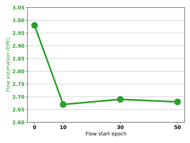
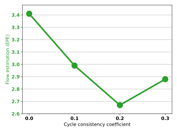
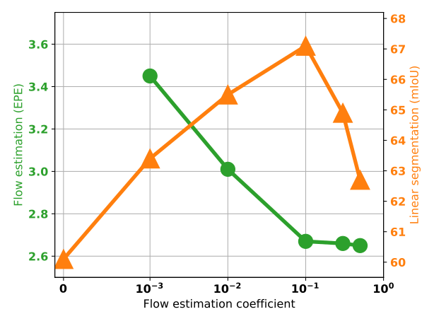
Training flow only above frozen image features is restrictive; optimizing the combined objectives or alternating at batch scale is more effective than large alternating phases. Starting the flow task after an initial content-learning warmup saves work and improves the tested recipe. Cycle consistency helps, but its coefficient matters. Too much motion-loss weight damages segmentation, so sharing an encoder does not remove the need to balance objectives.
5 Conclusion
Joint content and motion learning produces useful representations across the evaluated flow and segmentation tasks. Extending this result to larger natural-video collections, a shared training domain and longer-range dynamics remains future work. No action-conditioned planning result is claimed here.
A Implementation details
The training mixture samples video datasets throughout the run instead of repeatedly fine-tuning to each benchmark. Image self-supervision starts first, followed by flow learning. Layer normalization, bounded flow outputs and separate optimizer settings prevent unstable flow predictions from corrupting the combined loss.
A modified ConvNeXt-T encoder supplies six feature-pyramid levels. The reported recipe uses AdamW and eight V100 GPUs; the retained hyperparameter tables provide the exact batch sizes, schedules and separate encoder/estimator learning rates.
B Hyper-parameters
The appendix records dataset repetitions, input resolutions and loss coefficients. Motion-only tuning establishes flow settings before content-learning settings are tuned. Deeper feature levels receive stronger variance–covariance regularization. These tuned choices are part of the result and should be retained when attempting reproduction.
| Hyper-parameter | MC-JEPA | M-JEPA |
|---|---|---|
| data | ||
| ImageNet res. | (224, 224) | - |
| min_scale_crops | 0.08 | - |
| max_scale_crops | 1.0 | - |
| Sintel res. | (384, 832) | (384, 832) |
| KITTI res. | (256, 832) | (256, 832) |
| FlyingX res. | (384, 512) | (384, 512) |
| optimization | ||
| num_gpus | 8 | 8 |
| epochs | 100 | 100 |
| warmump_epochs | 10 | 10 |
| batch_size | 384 | - |
| optimizer | AdamW | AdamW |
| lr | - | |
| scheduler | cosine | cosine |
| end_lr | - | |
| weight_decay | - | |
| betas | (0.9, 0.999) | (0.9, 0.999) |
| architecture | ||
| drop_path_rate | 0.1 | 0.1 |
| layer_scale_init_value | 0.0 | 0.0 |
| expander dims. | 8192-8192-8192 | - |
| flow | ||
| flow_alpha | 0.1 | 1.0 |
| flow_coeff | 1.0 | 1.0 |
| flow_clip_value | 128.0 | 256.0 |
| flow_start_epoch | 10 | 0 |
| flow_loss_smooth_factor | 75.0 | 75.0 |
| flow_cycle_consistency_coeff | 0.2 | 0.1 |
| flow_batch_size | 8 | 8 |
| flow_lr | ||
| flow_weigth_decay |
| Dataset | Size | Repetition |
|---|---|---|
| FlyingThings | 40302 | 1 |
| FlyingChairs | 22232 | 1 |
| KITTI raw | 42382 | 1 |
| KITTI 2012 train | 200 | 100 |
| KITTI 2012 multiview train | 3800 | 5 |
| KITTI 2012 val | 198 | 100 |
| KITTI 2012 multiview val | 3762 | 5 |
| KITTI 2015 train | 200 | 100 |
| KITTI 2015 multiview train | 3800 | 5 |
| KITTI 2015 val | 198 | 100 |
| KITTI 2015 multiview val | 3762 | 5 |
| Sintel raw. | 27858 | 1 |
| Sintel clean | 1041 | 5 |
| Sintel final | 1041 | 5 |
| HD1k | 1047 | 5 |
| Layer | Var | Cov | Invariance | Flow |
|---|---|---|---|---|
| Expander output | 25.0 | 1.0 | 1.0 | - |
| Encoder output (L1) | 0.01 | 0.04 | - | 1.0 |
| L2 | 0.01 | 0.04 | - | 1.0 |
| L3 | 0.01 | 0.001 | - | 1.0 |
| L4 | 0.01 | 0.0 | - | 1.0 |
| L5 | 0.001 | 0.0 | - | 0.1 |
| L6 | 0.0001 | 0.0 | - | 0.01 |
C Architecture details
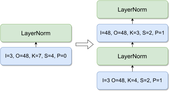
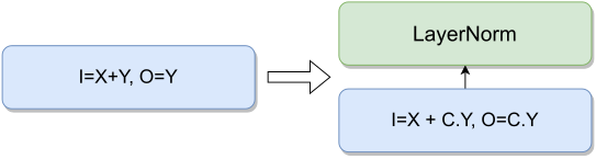
The encoder stem is modified to expose a finer feature pyramid for flow refinement. The flow estimator adds layer normalization after intermediate convolutions and increases channel capacity. Its final output layer avoids normalization, which could otherwise distort the range of physical displacement values. The original diagrams specify the architecture.
D Additional results
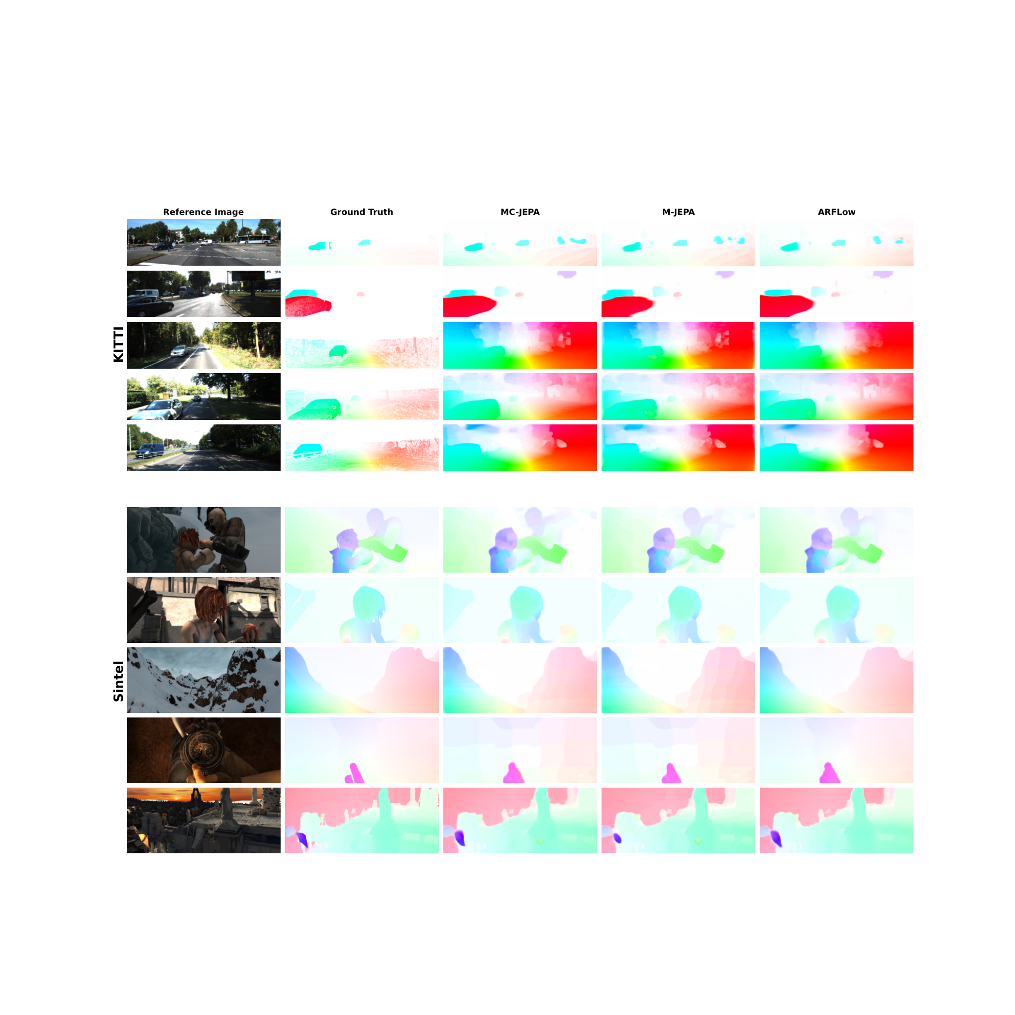
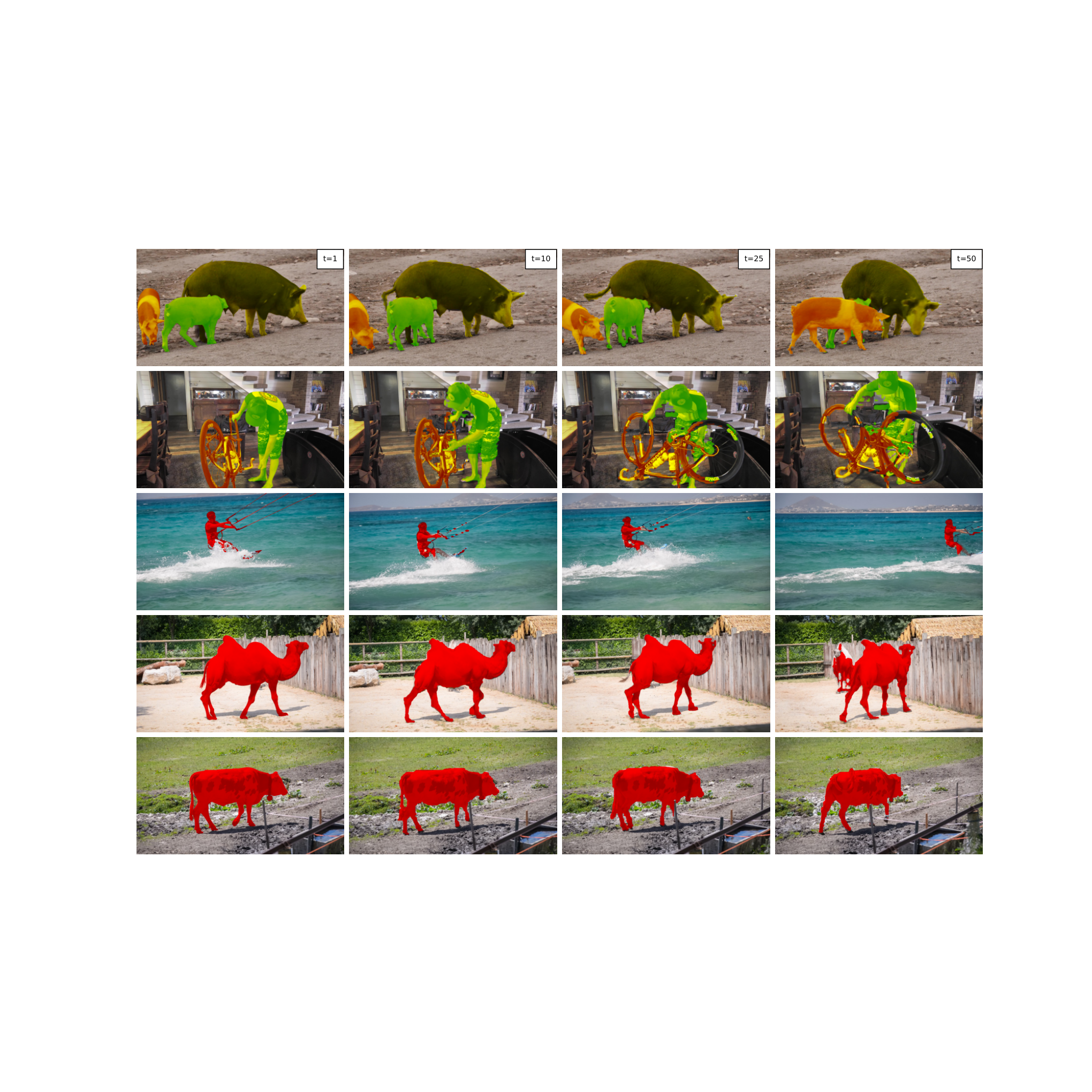
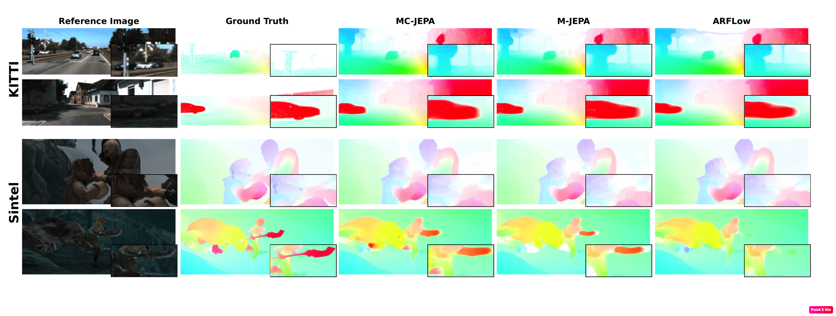
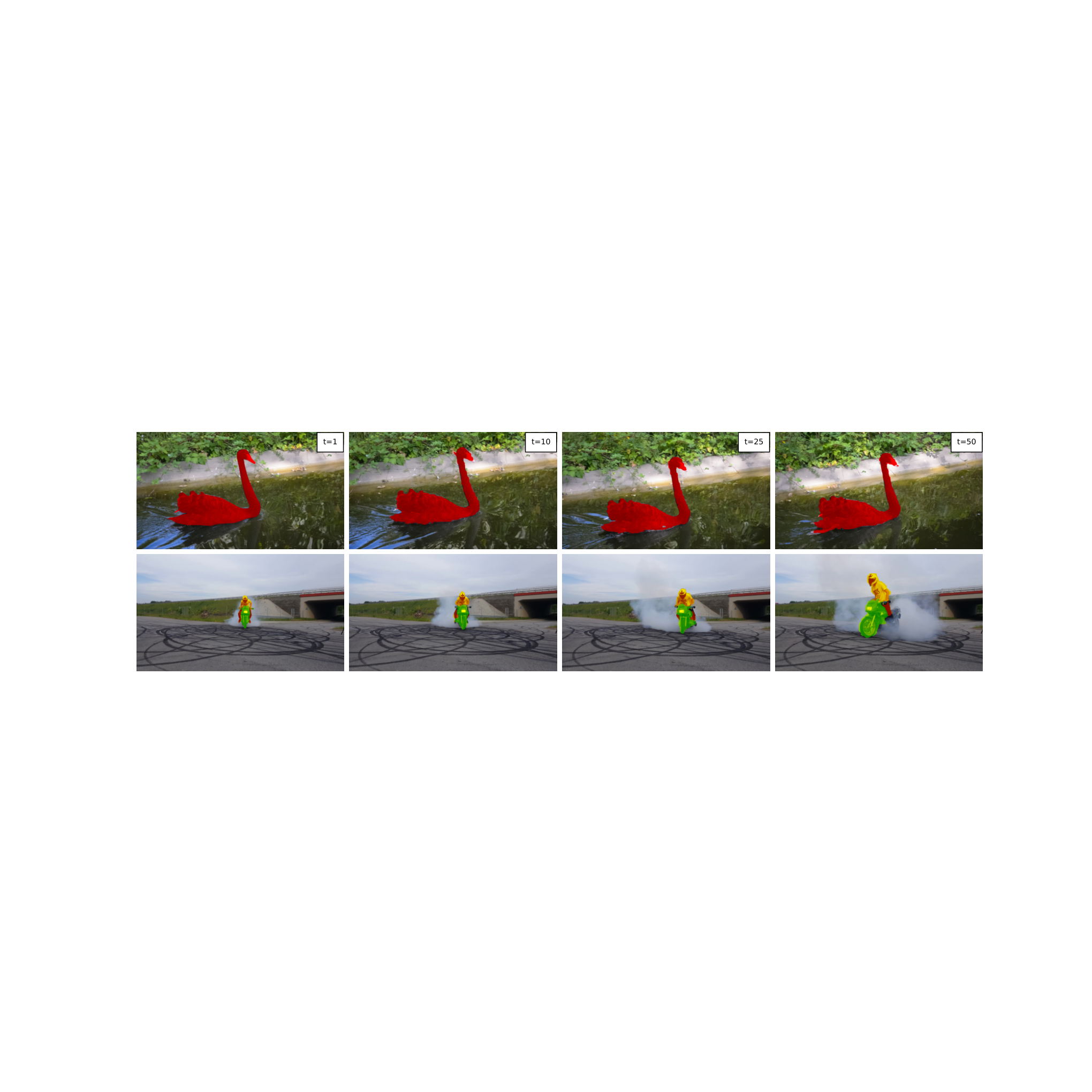
Additional tables separate the flow and video-segmentation metrics; the figures show qualitative successes and errors on both tasks. These supplement the numerical comparisons rather than establishing robustness outside the evaluated datasets.
E Additional ablation
Variance–covariance regularization is tested at the final layer and throughout the pyramid. Applying it at every level improves the reported motion and segmentation outcomes. A short regularization warmup also helps. Preventing complete collapse at one layer is therefore not the only concern: intermediate feature quality and stable optimization matter.
| Warmup ep. | Setup | K15 | clean | final | ISeg | VSeg | |
|---|---|---|---|---|---|---|---|
| - | None | 3.41 | 3.37 | 4.45 | 47.3 | 37.8 | |
| 0 | Last layer | 2.77 | 2.88 | 3.55 | 65.6 | 69.2 | |
| 0 | All layers | 2.65 | 2.80 | 3.48 | 66.2 | 69.4 | |
| 1 | All layers | 2.67 | 2.81 | 3.51 | 67.1 | 70.5 | |
| 2 | All layers | 2.91 | 2.99 | 3.78 | 62.5 | 64.1 |