Overview
This edition follows the complete arXiv v2, including the interpolation proof, bound visualization and both plotting-code appendices. Its title follows the PDF/HTML heading, “Position Interpolation”; the arXiv landing page uses “Positional Interpolation”.
At a glance
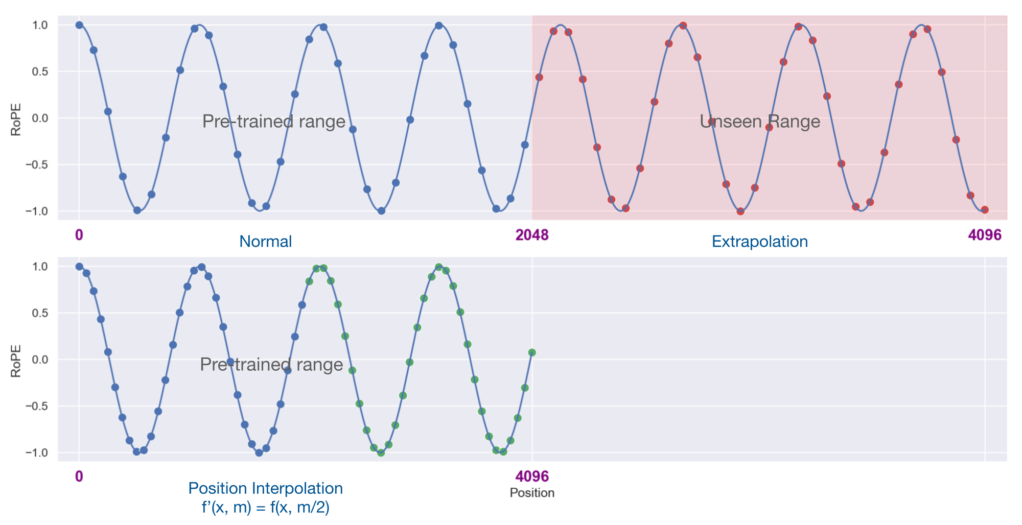
Intuition. A pretrained model has learned to interpret positions within a particular range. Position interpolation fits a longer sequence onto that familiar ruler. When doubling the window, position 6,000 is supplied to the rotary calculation as 3,000; the token itself is still present.
Reading the math. If the new length is s times the old length, position m becomes m/s. Neighboring tokens are consequently separated by 1/s of an old position unit, changing positional detail. Fine-tuning helps the model adapt to that denser ruler. This does not shorten the actual sequence or remove attention’s memory cost. Treat the reported experiments separately from the qualified theoretical bound.
Position Interpolation (PI) extends a pretrained rotary-position language model by shrinking its position indices into the original range, then fine-tuning on longer sequences. LLaMA experiments reach contexts up to 32,768 tokens with generally 1,000 fine-tuning steps. Long-text perplexity and passkey retrieval improve over the tested direct-extension baseline, with some degradation on short-context tasks. The paper’s approximately 600-fold theoretical bound comparison requires qualification because Appendix A contains an incorrect inequality.
1 Introduction
LLaMA was trained with 2,048-token context. Directly fine-tuning at greater lengths adapts slowly in the reported retrieval test. PI instead maps the new interval back into the trained positional interval, retaining the architecture and introducing no weights. The study tests long-text modeling, synthetic retrieval, short-context benchmarks and separately fine-tuned summarization. It acknowledges concurrent SuperHOT work; the experiments here use full fine-tuning rather than establishing a general low-rank-adaptation result.
2 Method
The method distinguishes increasing the number of tokens from extrapolating their numerical RoPE coordinates.
2.1 Background: Rotary Position Embedding (RoPE)
RoPE rotates query/key coordinate pairs at geometrically spaced frequencies. Their dot product is a sum of sinusoidal functions of relative displacement, weighted by content-dependent query/key products. Equations 1–2 retain the exact complex and real formulations.
Equations 1–2
| (1) |
| (2) | |||||
2.2 Direct Extrapolation
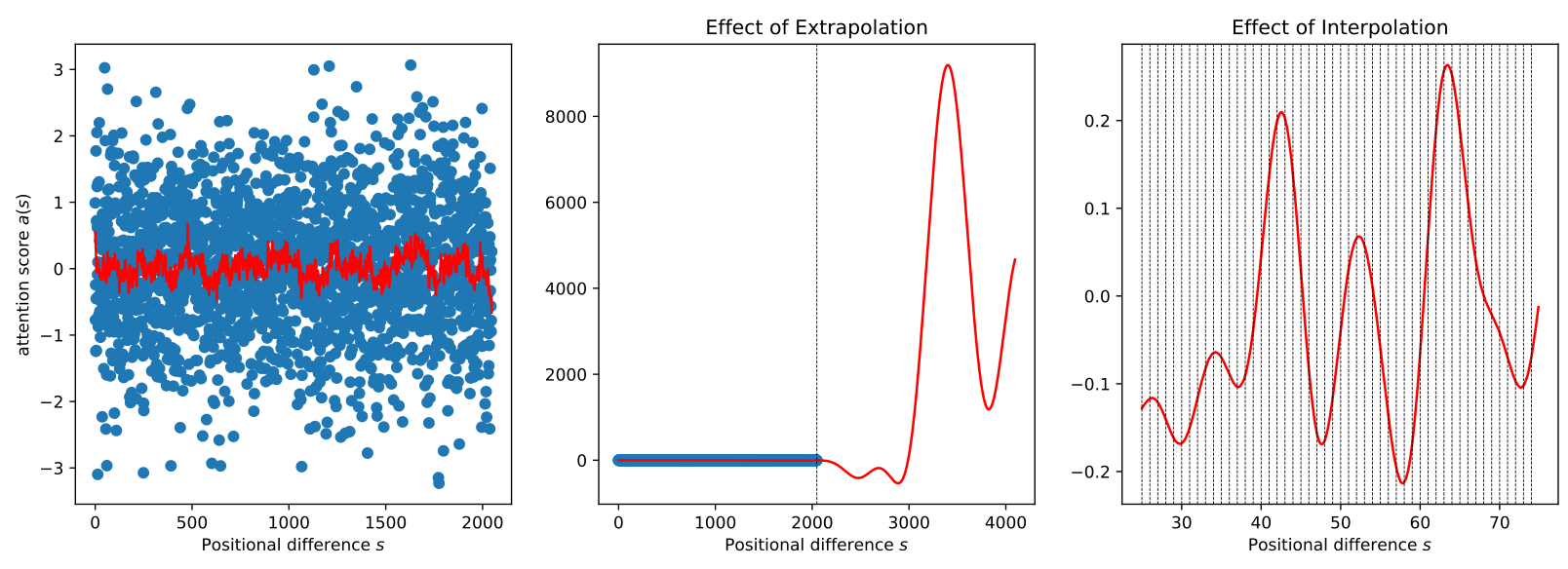
A trigonometric score that remains moderate on the trained interval can become large outside it. Figure 2 illustrates this with least-squares fits to random targets; it is a constructed function example, not a measurement of every trained attention head. An earlier distance-decay bound can still be large because its coefficient term depends on query/key magnitudes. Directly extending the tested original model produces perplexity above 1,000.
Equation 3
| (3) |
2.3 Proposed approach: Position Interpolation (PI)
For original length L and target length L′, replace position m by mL/L′ before applying RoPE. All relative coordinates remain within the original numerical range, although token density changes. Fine-tune with next-token prediction on longer inputs. The method changes neither weights’ shapes nor attention itself, so existing infrastructure remains usable; full attention still has its original long-sequence cost.
The source bounds deviation from linear interpolation between neighboring grid points and compares it with an extrapolation envelope. Its stated approximately 600× advantage is not a verified universal guarantee: Appendix A uses a reversed exponential inequality, and the extrapolation term is assessed numerically for selected settings. The original theorem and formulas remain below. Regularizing query/key product magnitudes is proposed as future work, not tested as an LLM-training method here.
Equation 4
| (4) |
Theorem 2.1 (Interpolation bound).
For attention score , where , its interpolation value for is bounded as follows:
Equation 5
| (5) |
where is the linear interpolation of two grid point and that are known to behave well, enforced by LLM pre-training:
Equation 6
| (6) |
Equations 7–8
| (7) |
| (8) |
3 Experiments
Reported configurations extend 2,048-token LLaMA to at most 32,768 tokens, a 16× extension. The source also says “32 times”, which is inconsistent with its displayed model settings. Model sizes do not all receive every target length.
3.1 Setup
Use LLaMA 7B, 13B, 33B and 65B with unchanged architecture. PI generally receives 1,000 next-token fine-tuning steps on the Pile; direct fine-tuning receives 10,000. AdamW uses betas (.9,.95), zero weight decay and twenty warmup steps from one-tenth the peak rate. Peak rate is 2×10⁻⁵ for 7B/13B and 10⁻⁵ for 33B/65B. The 7B–33B 8,192-token runs use 32 A100 GPUs and global batch 64; other configurations use 128 GPUs and batch 128, primarily for memory capacity. PyTorch FSDP and FlashAttention support training.
3.2 Long Sequence Language Modeling
Evaluate all 100 PG-19 test documents and 128 sampled Proof-pile documents of at least 32,768 SentencePiece tokens, truncating the latter to that length. Perplexity uses sliding windows with stride 256. PI benefits from longer context more than the direct fine-tuning baseline. For 7B at target length 16,384, full-window PG-19 perplexity falls from the original model’s 7.20 at 2,048 to 6.83; Proof-pile falls from 2.77 to 2.25.
The trend is not strictly monotone: for the 32,768-target 7B model, Proof-pile rises from 2.24 at evaluation length 16,384 to 2.48 at 32,768. Some short-window perplexities also regress. Without fine-tuning, PI’s 7B PG-19 perplexity is 16.10 at 8,192 and 112.13 at 16,384; after 200 steps these become 7.12 and 7.05, then 6.95 and 6.83 after 1,000 steps. Tables 1–3 preserve all configurations and intermediate results.
| Model | Evaluation Context Window Size | ||||||
|---|---|---|---|---|---|---|---|
| Size | Context Window | Method | 2048 | 4096 | 8192 | 16384 | 32768 |
| 7B | 2048 | None | 7.20 | ||||
| 7B | 8192 | FT | 7.21 | 7.34 | 7.69 | - | - |
| 7B | 8192 | PI | 7.13 | 6.96 | 6.95 | - | - |
| 7B | 16384 | PI | 7.11 | 6.93 | 6.82 | 6.83 | - |
| 7B | 32768 | PI | 7.23 | 7.04 | 6.91 | 6.80 | 6.77 |
| 13B | 2048 | None | 6.59 | - | - | - | - |
| 13B | 8192 | FT | 6.56 | 6.57 | 6.69 | - | - |
| 13B | 8192 | PI | 6.55 | 6.42 | 6.42 | - | - |
| 13B | 16384 | PI | 6.56 | 6.42 | 6.31 | 6.32 | - |
| 13B | 32768 | PI | 6.54 | 6.40 | 6.28 | 6.18 | 6.09 |
| 33B | 2048 | None | 5.82 | - | - | - | - |
| 33B | 8192 | FT | 5.88 | 5.99 | 6.21 | - | - |
| 33B | 8192 | PI | 5.82 | 5.69 | 5.71 | - | - |
| 33B | 16384 | PI | 5.87 | 5.74 | 5.67 | 5.68 | - |
| 65B | 2048 | None | 5.49 | - | - | - | - |
| 65B | 8192 | PI | 5.42 | 5.32 | 5.37 | - | - |
| Model | Evaluation Context Window Size | ||||||
|---|---|---|---|---|---|---|---|
| Size | Context Window | Method | 2048 | 4096 | 8192 | 16384 | 32768 |
| 7B | 2048 | None | 2.77 | - | - | - | - |
| 7B | 8192 | FT | 2.85 | 2.74 | 2.73 | - | - |
| 7B | 8192 | PI | 2.79 | 2.57 | 2.39 | - | - |
| 7B | 16384 | PI | 2.79 | 2.57 | 2.37 | 2.25 | - |
| 7B | 32768 | PI | 2.82 | 2.59 | 2.39 | 2.24 | 2.48 |
| 13B | 2048 | None | 2.66 | - | - | - | - |
| 13B | 8192 | FT | 2.71 | 2.56 | 2.50 | - | - |
| 13B | 8192 | PI | 2.67 | 2.47 | 2.30 | - | - |
| 13B | 16384 | PI | 2.68 | 2.47 | 2.29 | 2.18 | - |
| 13B | 32768 | PI | 2.68 | 2.46 | 2.28 | 2.15 | 2.35 |
| 33B | 2048 | None | 2.49 | - | - | - | - |
| 33B | 8192 | FT | 2.56 | 2.48 | 2.47 | - | - |
| 33B | 8192 | PI | 2.50 | 2.32 | 2.18 | - | - |
| 33B | 16384 | PI | 2.53 | 2.34 | 2.18 | 2.07 | - |
| 65B | 2048 | None | 2.42 | - | - | - | - |
| 65B | 8192 | PI | 2.43 | 2.26 | 2.12 | - | - |
| Model | Number of fine-tuning steps | ||||||
|---|---|---|---|---|---|---|---|
| Size | Context Window | 0 | 200 | 400 | 600 | 800 | 1000 |
| 7B | 8192 | 16.10 | 7.12 | 7.10 | 7.02 | 6.99 | 6.95 |
| 7B | 16384 | 112.13 | 7.05 | 6.93 | 6.88 | 6.84 | 6.83 |
3.3 Measuring Effective Context Window Size through Passkey Retrieval
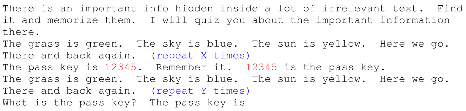
Hide a random five-digit passkey in repetitive irrelevant text, following Landmark Attention. Test ten trials at each of 32 uniformly spaced distances. The reported effective length is the greatest tested distance such that every shorter tested distance reaches at least 20% success—not perfect retrieval. PI reaches its target at 200 steps across the displayed configurations. Results are not uniformly stable: the 7B/32,768 run falls to 18,432 at 600 steps before recovering. Direct 7B fine-tuning reaches only 2,560 after 10,000 steps. Figure 3 retains the full prompt.
| Model | Fine-tuning steps | |||||||
| Size | Context Window | Method | 200 | 400 | 600 | 800 | 1000 | 10000 |
| 7B | 8192 | FT | 1792 | 2048 | 2048 | 2048 | 2304 | 2560 |
| 33B | 8192 | FT | 1792 | 2048 | 1792 | 2048 | 2304 | - |
| 7B | 8192 | PI | 8192 | 8192 | 8192 | 8192 | 8192 | - |
| 7B | 16384 | PI | 16384 | 16384 | 16384 | 16384 | 16384 | - |
| 7B | 32768 | PI | 32768 | 32768 | 18432 | 32768 | 32768 | - |
| 33B | 8192 | PI | 8192 | 8192 | 8192 | 8192 | 8192 | - |
| 33B | 16384 | PI | 16384 | 16384 | 16384 | 16384 | 16384 | - |
Selectable original prompt
There is an important info hidden inside a lot of irrelevant text. Find it and memorize them. I will quiz you about the important information there.
The grass is green. The sky is blue. The sun is yellow. Here we go. There and back again. (repeat X times)
The pass key is 12345. Remember it. 12345 is the pass key.
The grass is green. The sky is blue. The sun is yellow. Here we go. There and back again. (repeat Y times)
What is the pass key? The pass key is
3.4 Benchmarks on Original Context Window Size
Table 5 evaluates original-window zero-shot tasks. The 7B 8,192-target Pile model drops BoolQ from 76.1 to 73.2, a 2.9-point loss, despite the source’s “up to 2%” summary. At 32,768, BoolQ falls to 64.7 and other scores also decline. The 33B/8,192 results are closer to baseline. A RedPajama comparison gives a different task-wise pattern; this small comparison does not establish that adaptation data never matters.
| Model Size | Context Window | Fine-tune on | BoolQ | PIQA | Race-M | Race-H | WinoGrande |
|---|---|---|---|---|---|---|---|
| 7B | 2048 | None | 76.1 | 78.9 | 55.7 | 42.2 | 69.6 |
| 7B | 8192 | Pile | 73.2 | 78.2 | 53.8 | 41.7 | 69.0 |
| 7B | 16384 | Pile | 69.8 | 77.6 | 53.3 | 40.9 | 67.8 |
| 7B | 32768 | Pile | 64.7 | 77.2 | 50.1 | 39.6 | 66.9 |
| 7B | 8192 | RedPajama | 75.5 | 77.4 | 54.5 | 41.5 | 68.1 |
| 33B | 2048 | None | 81.6 | 80.2 | 61.1 | 45.9 | 76.2 |
| 33B | 8192 | Pile | 80.2 | 80.7 | 60.2 | 45.7 | 75.9 |
3.5 Long Document Summarization
GovReport supplies 17,457 training and 972 evaluation documents. Starting from a PI-extended 16,384-context model, truncate documents to 15,000 tokens and summaries to 1,000, then fine-tune for ten additional epochs with loss only on summary tokens. Generate at temperature .5 and top-p .95, capped at 1,000 tokens. LLaMA-7B scores ROUGE-1/2/L 60.0/28.0/29.5: ROUGE-1 lies between CoLT5 Base and XL, while ROUGE-2/L are below both. This is a separately supervised summarization result, not zero-shot performance obtained from the 1,000-step context adaptation alone.

Selectable original prompt
Read the following article and then summarize it.
# .... Document goes here
Now summarize the above article.
Summary:
| Model | Evaluation Score | |||
| Model | Context Window | ROUGE-1 | ROUGE-2 | ROUGE-L |
| CoLT5 Base (Ainslie et al., 2023) | 16K | 58.7 | 29.6 | 31.4 |
| CoLT5 XL (Ainslie et al., 2023) | 16K | 61.3 | 32.2 | 33.8 |
| LLaMA-7B Extended | 16K | 60.0 | 28.0 | 29.5 |
4 Related Work
PI can complement retrieval by fitting more retrieved text in context. Recurrent/compressed-memory approaches trade access to past detail for lower cost; PI retains full attention over the longer input. Sparse or approximate attention addresses a different computational issue. Unlike methods requiring a new positional scheme during pretraining, PI targets existing rotary models. Vision Transformer interpolation resizes learned position embeddings; PI rescales continuous position indices without adding learned entries. Application to other position schemes is proposed future work.
5 Conclusions
Rescaling rotary coordinates plus brief fine-tuning makes substantially longer context usable in the tested LLaMA models. The evidence supports an economical adaptation of existing checkpoints, with explicit limits: full-attention cost remains, model/length coverage is uneven, short-context quality can decline and synthetic retrieval uses a low success threshold. Broader positional schemes and the source’s exact theoretical constant remain unresolved here.
Acknowledgements
The authors thank Mike Lewis for input on evaluation.
Appendix A Proof
The proof attempts to bound interpolation error using Taylor remainders and a bound on the second derivative of the trigonometric score. Equations 9–17 remain exactly as printed. The finite geometric series in Equation 13 is written without its numerator, and the next step uses cˣ≤1+x ln c, whereas convexity gives cˣ≥1+x ln c. Thus the stated d/(4 ln c) derivative bound and resulting numerical constant do not follow from this proof as written. This does not negate the experimental comparisons or the general motivation for keeping positions within the trained range.
Equations 9–17
| (9) | |||||
| (10) |
| (11) |
| (12) | |||||
| (13) |
| (14) |
| (15) |
| (16) |
| (17) |
Appendix B Visualization of quantities in extrapolation bound
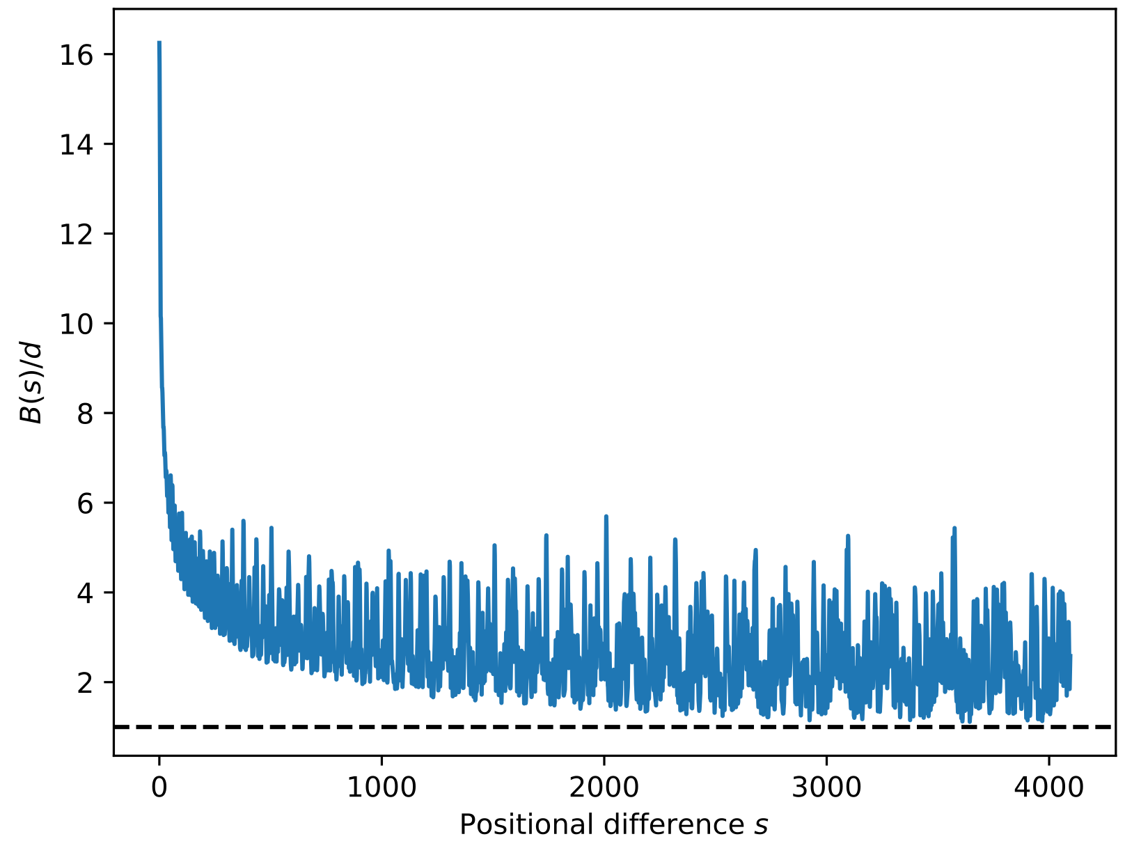
Figure 5 evaluates the partial-phase-sum term B(s)/d with c=10,000 and head dimension 128, the LLaMA-7B setting. Its oscillatory envelope is typically above one over the plotted range. This numerical illustration explains why the earlier extrapolation bound can be loose; it is not a proof for every displacement or configuration.
Appendix C Code
The original two code listings are retained with line breaks and indentation. They generate the illustrative fit and bound plots, not model-training experiments.
C.1 Code for Fig. 2
Construct sine/cosine features for 2,048 positions with dimension 128, fit random targets by solving the unregularized normal equations, then plot extrapolation to 4,096 and interpolation on a finer grid. The example is sensitive to numerical conditioning and the random sample. The source listing remains unchanged, including the loop that draws the interpolation grid.
# build basis function
d = 4096 // 32
theta = 10000
# Frequency computation,
freqs = 1.0 / (theta ** (torch.arange(0, d, 2)[: (d // 2)].float() / d))

# construct basis function
L = 2048

x = torch.zeros(L)
x[:L] = torch.arange(0, L)

# basis functions
xfreq = torch.outer(x, freqs)

y = torch.randn(x.shape[0])

# do linear regression
X = torch.cat([xfreq.sin(), xfreq.cos()], dim=1)

eps = 0.000
coeffs = torch.linalg.solve(X.t() @ X + torch.eye(X.shape[1]) * eps, X.t() @ y)

x2 = torch.arange(0, 2*L)
xfreq2 = torch.outer(x2, freqs)
X2 = torch.cat([xfreq2.sin(), xfreq2.cos()], dim=1)

y2 = X2 @ coeffs

x3 = torch.arange(25, 75, 0.125)
xfreq3 = torch.outer(x3, freqs)
X3 = torch.cat([xfreq3.sin(), xfreq3.cos()], dim=1)

y3 = X3 @ coeffs

plt.figure(figsize=(16,5))

plt.subplot(1, 3, 1)
plt.plot(x2[:L], y2[:L], "r")
plt.scatter(x, y)
plt.ylabel("attention score $a(s)$")
plt.xlabel("Positional difference $s$")

plt.subplot(1, 3, 2)

plt.plot(x2, y2, "r")
plt.scatter(x, y)
plt.axvline(L, color="k", linestyle="--", linewidth=0.5)

plt.title("Effect of Extrapolation")
plt.xlabel("Positional difference $s$")


plt.subplot(1, 3, 3)
plt.plot(x3, y3, "r")
for i in range(25,75):
    plt.axvline(i, color="k", linestyle="--", linewidth=0.5)
plt.title("Effect of Interpolation")
plt.xlabel("Positional difference $s$")
plt.show()
C.2 Code for Fig. 5
Compute cumulative complex-phase magnitudes and plot their sum divided by d over 4,096 displacements. The printed listing contains typographic quotation marks around k in the color argument; these source characters are preserved rather than silently converted into executable code.
L = 2048
x = torch.arange(0, 2*L)
d = 4096 // 32
theta = 10000
freqs = 1.0 / (theta ** (torch.arange(0, d, 2)[: (d // 2)].float() / d))

xfreq = torch.outer(x, freqs)

mags = (xfreq.sin().cumsum(dim=1).pow(2) + xfreq.cos().cumsum(dim=1).pow(2)).sqrt()

plt.plot(mags.sum(dim=1)/d)
plt.axhline(1.0, color=’k’, linestyle="--")
plt.xlabel("Positional difference $s$")
plt.ylabel("$B(s)/d$")
plt.show()