The complete article and network-hyperparameter appendix are condensed below. All numbered figures, scientific tables, displayed equations, and original author portraits are retained.
Guangming Wang received the B.S. degree from Department of Automation from Central South University, Changsha, China, in 2018, and Ph.D. degree in Control Science and Engineering from Shanghai Jiao Tong University, Shanghai, China. He visited Department of Computer Science of ETH Zurich from 2022 to 2023. He is currently a Research Associate with the Department of Engineering, University of Cambridge, UK. His current research interests include robot perception, localization, and mapping.
Yu Zheng
received the B.Eng degree in Department of Artificial Intelligence, Shanghai Jiao Tong University, China, in 2023. He is currently pursuing the Ph.D. degree in Control Science and Engineering with Shanghai Jiao Tong University, China. His current research interests include SLAM and computer vision.
Yuxuan Wu received the B.Eng degree in School of Astronautics, Beihang University. He is currently pursuing the Ph.D. degree in Control Science and Engineering with Shanghai Jiao Tong University, China. Her latest research interests include SLAM and computer vision.
Yanfeng Guo
received his B.Eng degree at Department of Automation from Shanghai Jiao Tong University, Shanghai, China, in 2022. He is currently pursuing the M.S degree in Electrical and Computer Engineering at University of California, Los Angeles, the United States. His current research interests include computer vision and autonomous driving system.
Zhe Liu received his B.S. degree in Automation from Tianjin University, Tianjin, China, in 2010, and Ph.D. degree in Control Technology and Control Engineering from Shanghai Jiao Tong University, Shanghai, China, in 2016. From 2017 to 2020, he was a Post-Doctoral Fellow with the Department of Mechanical and Automation Engineering, The Chinese University of Hong Kong, Hong Kong. From 2020 to 2022, he was a Research Associate of Department of Computer Science and Technology, University of Cambridge, United Kingdom. He is currently a tenure-track associate professor of Institute of Artificial Intelligence, Shanghai Jiao Tong University. His research interests include scheduling and optimization of large-scale robotic systems, resilient navigation of industrial self-driving systems, localization of self-driving systems, coordination of multi-robot formations, and robot control.
Yixiang Zhu
received his B.Eng degree at Department of Electrical Engineering from Shanghai Jiao Tong University, Shanghai, China, in 2023. He is currently pursuing the M.S degree in Computer Control and Automation at Nanyang Technological University, Singapore. His current research interests include SLAM and computer vision.
Wolfram Burgard
is Vice President for Automated
Driving Technology at the Toyota Research Institute
in Los Altos, USA. He is on leave from a Professorship for Computer Science at the University of
Freiburg, Germany where he heads the Laboratory
for Autonomous Intelligent Systems. He received his
Ph.D. degree in computer science from the University
of Bonn in 1991. His areas of interest lie in robotics
and artificial intelligence. In the past, Wolfram
Burgard and his group developed several innovative
probabilistic techniques for robot navigation and
control. They cover different aspects including localization, mapping, path
planning, and exploration. For his work, Wolfram Burgard received several
best paper awards from outstanding national and international conferences.
In 2009, Wolfram Burgard received the Gottfried Wilhelm Leibniz Prize, the
most prestigious German research award. In 2010 he received the Advanced
Grant of the European Research Council. Wolfram Burgard is the spokesperson
of the Cluster of Excellence BrainLinks-BrainTools, President of the IEEE
Robotics and Automation Society, and fellow of the AAAI, EurAi and IEEE.
Hesheng Wang
received the B.Eng. degree in electrical engineering from the Harbin Institute of Technology, Harbin, China, in 2002, and the M.Phil. and Ph.D. degrees in automation and computer-aided engineering from The Chinese University of Hong Kong, Hong Kong, in 2004 and 2007, respectively. He is currently a Professor with the Department of Automation, Shanghai Jiao Tong University, Shanghai, China. His current research interests include visual servoing, service robot, computer vision, and autonomous driving.
Dr. Wang is an Associate Editor of IEEE Transactions on Automation Science and Engineering, IEEE Robotics and Automation Letters, Assembly Automation and the International Journal of Humanoid Robotics, a Technical Editor of the IEEE/ASME Transactions on Mechatronics, an Editor of Conference Editorial Board (CEB) of IEEE Robotics and Automation Society. He served as an Associate Editor of the IEEE Transactions on Robotics from 2015 to 2019. He was the General Chair of IEEEROBIO 2022 and IEEERCAR 2016, and the Program Chair of the IEEEROBIO 2014 and IEEE/ASMEAIM 2019. He will be the General Chair of IEEE/RSJIROS 2025.
At a glance
I2PNet learns to register a camera image directly with a raw LiDAR point cloud. Soft cross-modal correspondences, learned outlier weights, and iterative pose refinement are optimized together under pose supervision. Experiments cover large and small initial misalignments, transfer across driving and ground-robot datasets, and simulated camera–LiDAR miscalibration. The method needs known camera intrinsics and a relevant local point-cloud map; it does not solve city-scale place recognition.
I Introduction
A robot can use an economical monocular camera to localize against a map built previously with LiDAR. The difficult step is matching texture-rich image pixels to geometry-rich three-dimensional points. Earlier pipelines separately learn correspondences and solve pose, or turn points into a depth image that loses useful geometry under large initial misalignment. I2PNet instead retains raw point structure and connects feature extraction, association, outlier handling, and pose regression through a common supervised objective. Its normalized image-plane representation accommodates different supplied camera calibrations.
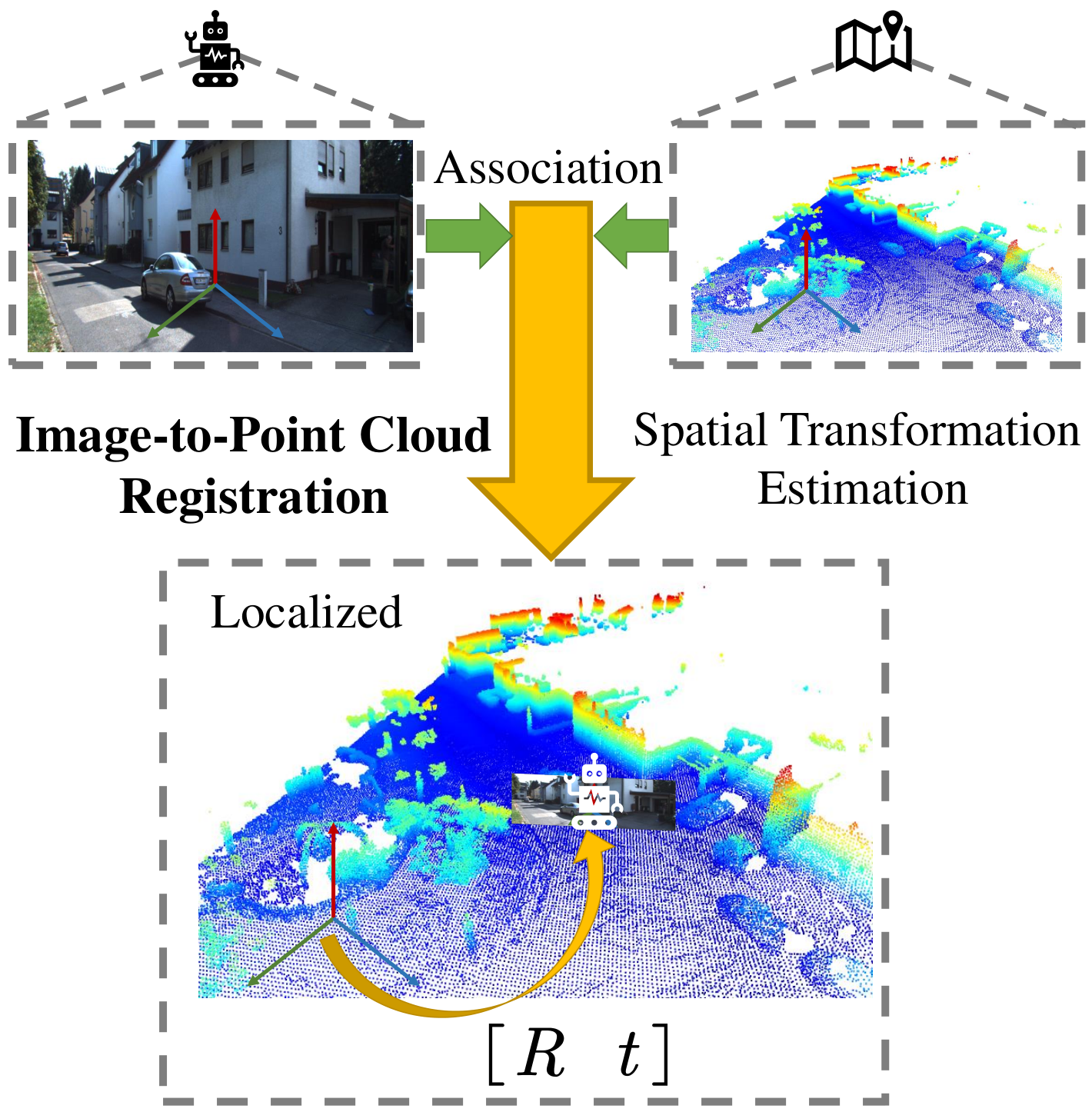
Figure 1: The pipeline of monocular camera localization in LiDAR maps with image-to-point cloud registration. Image-to-point cloud registration associates the image and point cloud and estimates the spatial transformation between them. With the estimated transformation, the pose of the monocular camera in the LiDAR map is obtained and the robot is localized.
II Related Work
Prior work separates cross-modal localization from the related task of correcting a camera–LiDAR sensor transform.
II-A Image-to-Point Cloud Registration for Robot Localization
Feature matching followed by a perspective-n-point or inverse-projection solver can localize over large displacements, but its stages are not jointly optimized. Depth-image methods such as CMRNet allow end-to-end refinement yet lose projected points when the initial alignment is poor. I2PNet combines raw-point feature extraction with differentiable association and direct pose prediction, avoiding a separate iterative geometric solver.
Calibration methods match contours or intensities, or learn alignment between camera and depth images. RegNet, CalibNet, and RGGNet emphasize different feature and loss designs. I2PNet applies the same raw-point/image registration architecture to both localization and synthetic extrinsic-calibration errors.
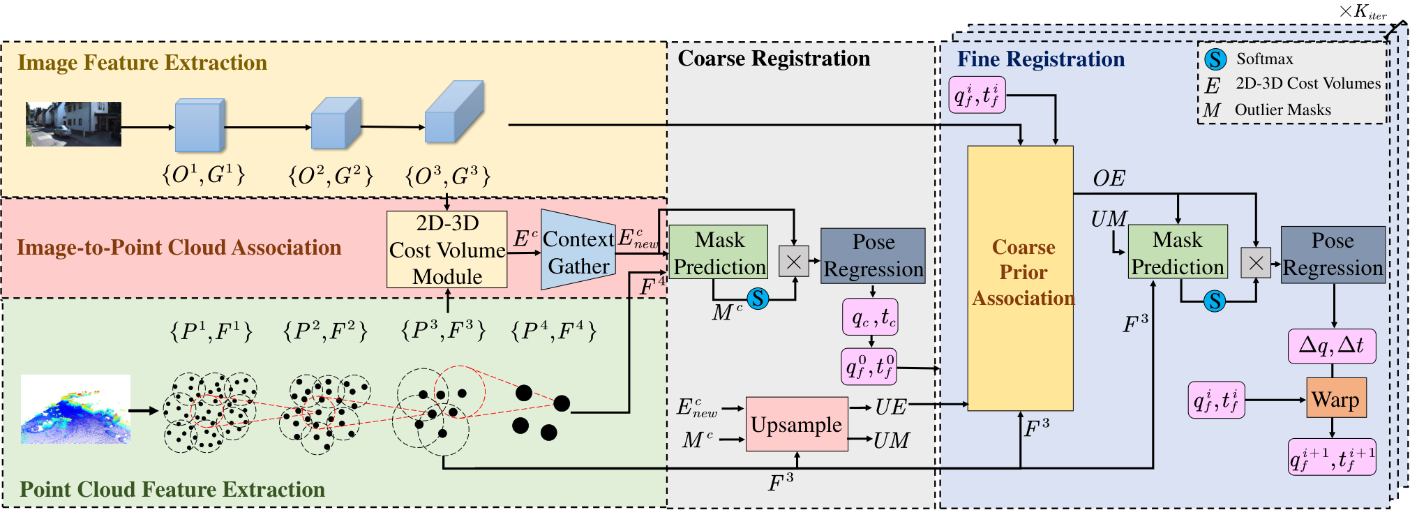
Figure 2: The outline of I2PNet. I2PNet takes the RGB image and the raw LiDAR point cloud as input. Through the feature extraction pyramid, coarse registration, and fine registration, the network finally predicts relative pose between the image and point cloud. The detailed structure of coarse prior association is shown in Fig. 3.
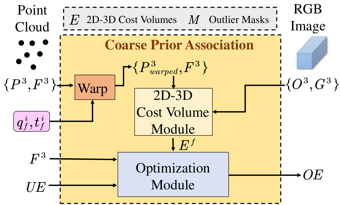
Image and point-cloud pyramids provide multiscale features. Coarse association produces a pointwise cost volume; spatial context and learned outlier weights aggregate it into a rotation quaternion and translation. Fine registration warps points by the current estimate, recomputes more local correspondences, combines them with upsampled coarse information, and predicts a residual transform. Repeating this refinement trades inference time for accuracy.
Figure 3: The detailed structure of the coarse prior association in Fig. 2.
III-B Feature Extraction
III-B 1 Image Feature Extraction
Three image-pyramid levels each contain five convolutional blocks with normalization, leaky rectification, and pooling. The network retains feature vectors and the corresponding pixel coordinates.
III-B 2 Point Cloud Feature Extraction
PointNet++-style aggregation builds four point-feature levels. For single rotating-LiDAR scans, spherical coordinates permit stride sampling and a restricted two-dimensional search window; three-dimensional nearest-neighbor selection then occurs within that window. This replaces expensive full-cloud sampling and search while preserving raw three-dimensional features. A distance threshold rejects remote neighbors. Accumulated maps used in the small-range experiment instead require ordinary PointNet++ sampling.
Equations 1–2
(1)
(2)
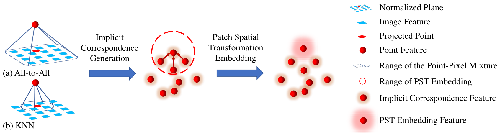
Figure 4: The process diagram of the 2D-3D cost volume module. The Implicit Correspondence (IC) generation module uses an all-to-all or KNN-based point-pixel mixture to match the points and pixels on the normalized plane of the pinhole camera model. Then, the similarities of each point-pixel pair are calculated and aggregated to generate the point-wise IC features. Based on the IC features, the Patch Spatial Transformation (PST) embedding module aggregates the IC features of the neighbors of each point to estimate the patch spatial transformation information and embeds it in the PST embedding features. The module finally outputs the PST embedding features as the 2D-3D cost volumes.
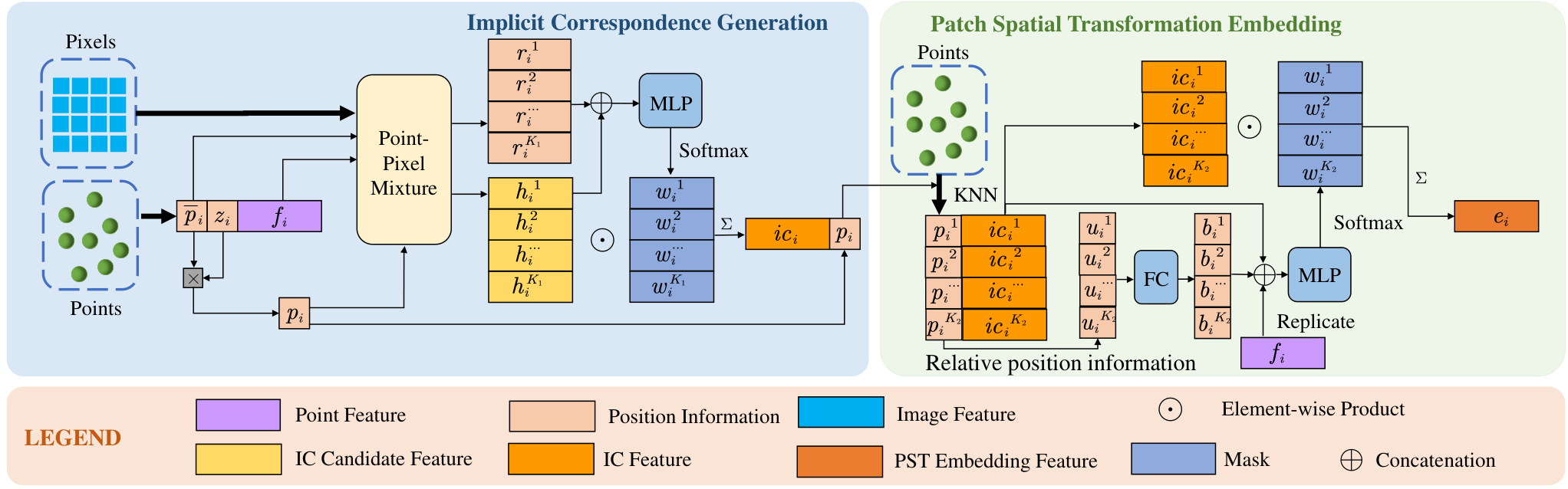
Figure 5: The detailed pipeline of the 2D-3D cost volume module. Given the features of the image and point cloud, as well as their position information, the module estimates the PST embedding features as the 2D-3D cost volumes. The detailed structures of the point-pixel mixtures are shown in Fig. 6 and Fig. 7.
Points project to a normalized pinhole plane, and image pixels map to that plane using the inverse camera-intrinsic matrix. Learned soft matching yields implicit correspondence features; aggregation over neighboring points adds patch-transform information. Intrinsic-independent coordinates therefore do not mean that camera intrinsics are unknown or unnecessary.
III-C 2 Detailed Pipeline
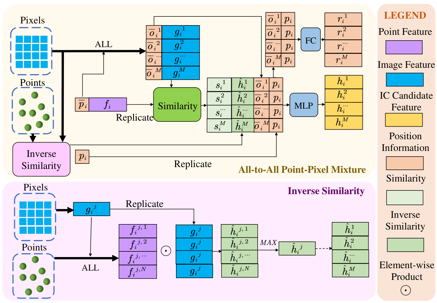
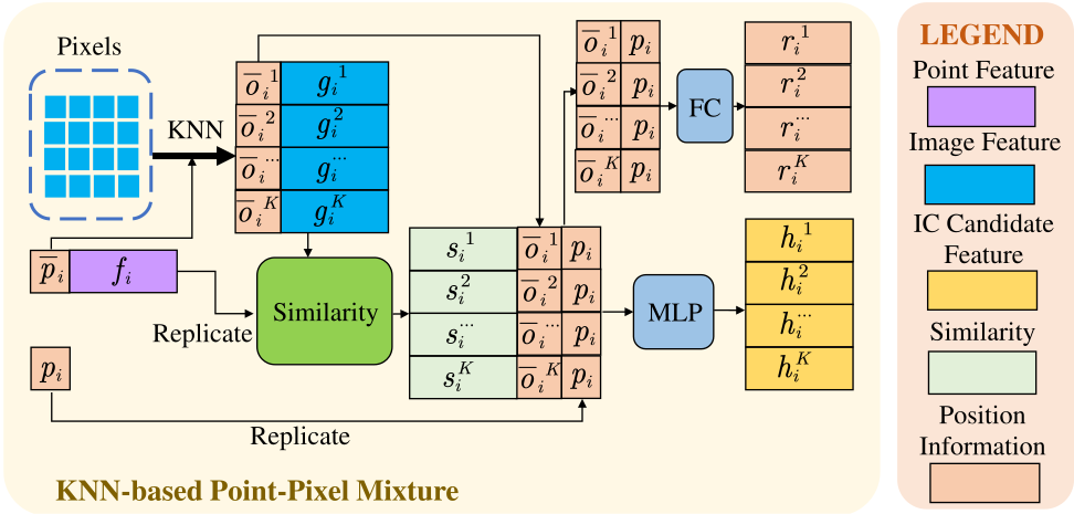
Large initial errors use all image features as coarse matching candidates, then nearest pixels during refinement; small-error tasks use local candidates at both stages. Channelwise normalized point/image feature products measure similarity. The all-to-all version also includes an inverse-match feature to reduce ambiguous associations. Position-aware attention forms a soft weighted correspondence feature for each point. A second neighborhood aggregation incorporates absolute positions, offsets, and distances, producing a patch spatial transformation embedding used as the cost volume. These learned features encode evidence for alignment rather than explicit, guaranteed-correct point matches.
Equations 3–4
(3)
(4)
Figure 6:
The all-to-all point-pixel mixture for the coarse registration. The all-to-all mixture treats all the pixels as the correspondence candidates of the point. In addition, the inverse similarity is adopted for robust correspondence generation.Equations 5–8
(5)
(6)
(7)
(8)
Figure 7: The KNN-based point-pixel mixture. This type of point-pixel mixture treats the nearest pixel neighbors as the pixel correspondence candidates. Equations 9–14
(9)
(10)
(11)
(12)
(13)
(14)
III-D Coarse Registration
III-D 1 Context Gathering Module
A further point-neighborhood aggregation pools coarse cost-volume context using the fourth point-pyramid level. This lets surrounding associations influence each point’s transformation evidence.
Equation 15
(15)
III-D 2 Outlier Mask Prediction Module
A shared network combines point appearance/geometry features with contextual cost volumes to predict outlier scores. Points outside the image view, or with unreliable correspondences, should receive less influence on pose.
Equation 16
(16)
III-D 3 Pose Regression
Softmax-normalized outlier scores weight the cost-volume sum. Fully connected layers and training-time dropout decode this global feature into translation and a normalized quaternion. Learned weighting replaces a separate consensus-based outlier solver; it does not provide a geometric correctness certificate.
Equations 17–18
(17)
(18)
III-D 4 Upsampling Layer
Two separate neighborhood-based upsampling modules transfer coarse cost volumes and outlier masks to the finer point set. Each combines relative coordinates, pooled coarse features, and fine point features.
Equations 19–20
(19)
(20)
III-E Fine Registration
III-E 1 Pose Warping
The current quaternion and translation transform the fine-level point coordinates. Nearest-pixel association on these warped coordinates estimates the remaining image–point misalignment.
Equation 21
(21)
III-E 2 Optimization Module
Shared networks fuse fresh fine cost volumes with upsampled coarse volumes and point features. A parallel fusion predicts refined outlier masks from the optimized cost volumes, earlier masks, and point features.
Equations 22–23
(22)
(23)
III-E 3 Pose Refinement
The weighted pose decoder estimates a residual rotation and translation. Quaternion composition and the corresponding translation update refine the current transform; the equations retain the composition order.
Equations 24–26
(24)
(25)
(26)
III-F Loss Function
Supervised quaternion and translation errors train both coarse and fine predictions. Learned scale parameters balance their different units. Training uses one refinement iteration for efficiency, with a weighted sum of the two registration losses.
Equations 27–28
(27)
(28)
IV Experiments
Evaluation separates two different localization protocols and examines transfer, component ablations, runtime, and refinement depth.
IV-A Implementation Details
Experiments use an RTX 3090, Adam, batch size eight, initial learning rate 0.001 with 1% decay per epoch, and 0.5 pose-decoder dropout. Point features are extracted in the LiDAR frame. Comparisons use one fine iteration. Large-range perturbations cover full yaw and up to 10 m of ground-plane translation; small-range perturbations independently vary each rotation axis within ±10° and each translation axis within ±2 m. These settings are not equivalent global-localization problems.
Table I: Large-Range Localization Error on the KITTI Odometry and NuScenes Datasets
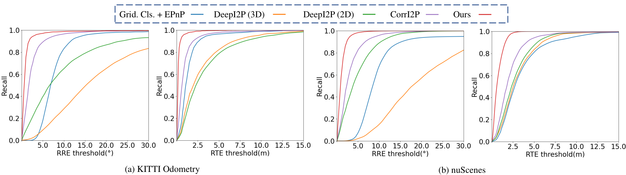
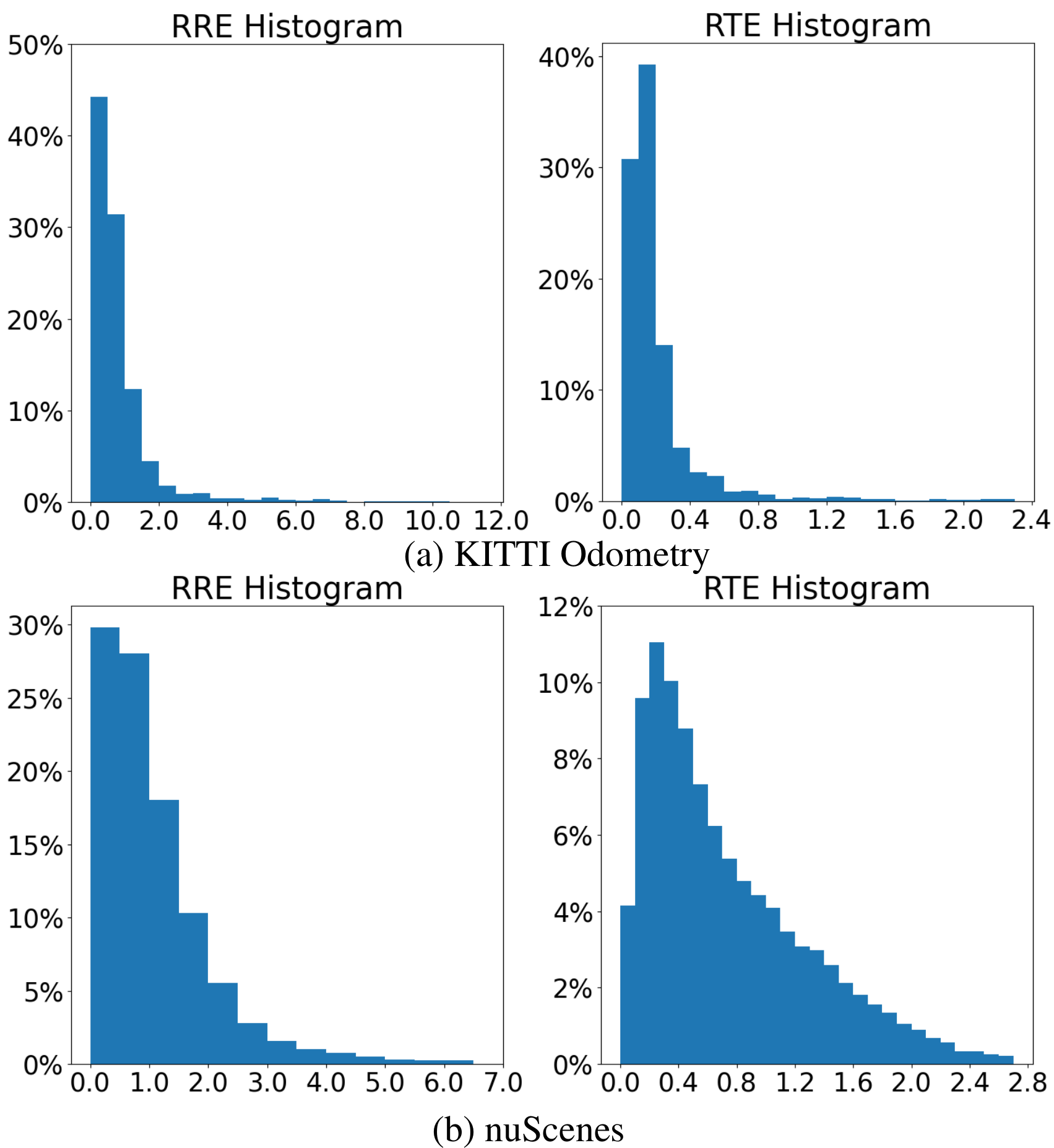
Figure 8: The registration recall curves of the methods with different RTE and RRE thresholds on KITTI Odometry and nuScenes datasets. The y-axis (recall) of the recall curve presents the success rate that RREs or RTEs are less than the threshold in the x-axis.Figure 9: The histograms of RTE and RRE on the KITTI Odometry and nuScenes datasets. The x-axis is the RTE (m) or RRE (∘), and the y-axis is the percentage falling into the corresponding bin. The bin size of RRE and RTE is and respectively.
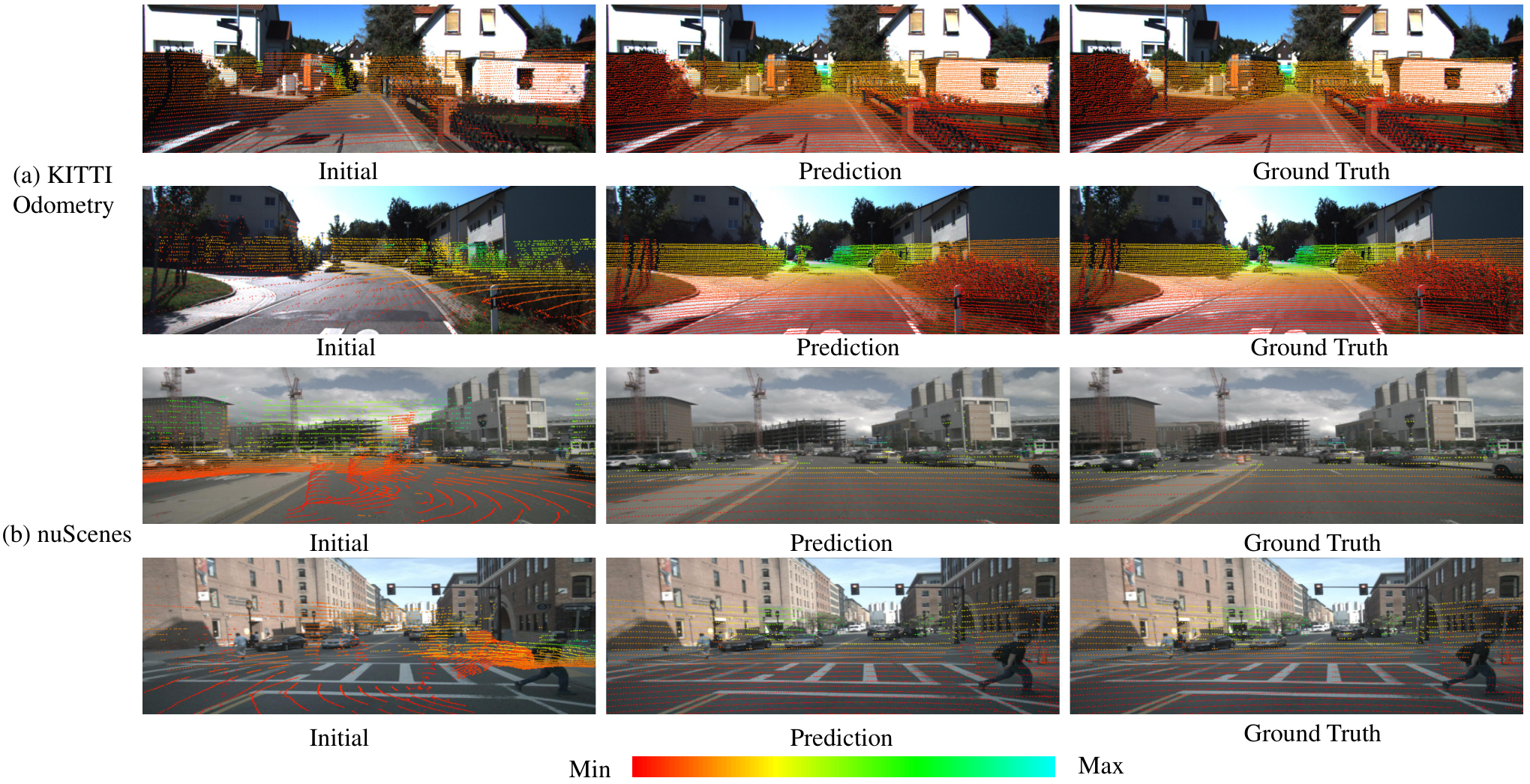
Figure 10: Visualization of large-range localization results on KITTI Odometry and nuScenes datasets. This figure presents the large-range localization results on the KITTI Odometry and nuScenes datasets through the visualization of image-to-point cloud registration. The color bar shows the depth of each LiDAR point.
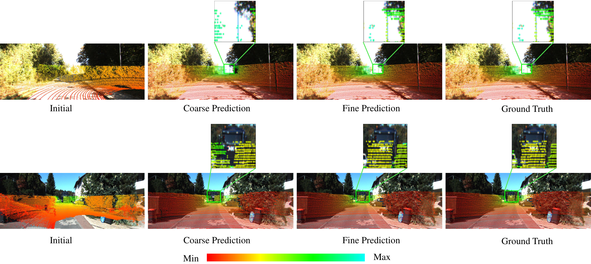
Figure 11: Visualization of coarse and fine registration results. The coarse and fine predictions are obtained from the coarse and fine registration respectively. The zoom-in views of the areas marked by the bounding boxes in each picture are to better present the difference among the coarse prediction, fine prediction, and ground truth. The color bar has the same meaning as Fig. 10.
IV-B Large-Range Localization
IV-B 1 Dataset and Data Pre-processing
KITTI sequences 0–8 train the large-range model and 9–10 test it; nuScenes uses 850/150 traversals. A same-frame KITTI scan, or a pose-aligned nearby nuScenes scan, is transformed synthetically to create each localization example. Cropped images resize to 160×512 or 160×640; all scan points are supplied. Initial features contain intensity plus estimated normals for KITTI, or intensity plus zero placeholders for nuScenes. Thus this protocol mainly tests registration of a perturbed scan, with known pairing to the image.
IV-B 2 Experimental Results and Visualization
Mean errors are reported only for samples below both 10° rotation error and 5 m translation error; recall curves expose failures omitted by those conditional means. I2PNet reports 0.83°/0.21 m on KITTI and 1.13°/0.75 m on nuScenes, versus CorrI2P’s 2.07°/0.74 m and 2.65°/1.83 m. Qualitative overlays and coarse/fine comparisons show improved alignment. These numbers should be read together with the recall curves and the synthetic perturbation protocol.
Equation 29
(29)
IV-B 3 Validation on Non-Car-Like Platform
M2DGR evaluates a ground robot across outdoor, hall, elevator, and room scenes. When trained and tested on that dataset, I2PNet reports 0.89–1.70° rotation error and 0.24–0.36 m translation error across the four scene types, outperforming the listed baselines.
Table II: Large-Range Localization Evaluated on M2DGR Dataset. All Models Are Trained and Tested on M2DGR Dataset to Demonstrate the Performance on a Non-Car-Like Platform, a Ground Robot Platform
Table III: Generalization Experiments from KITTI Odometry Dataset to NuScenes and M2DGR Datasets. All Models Are Trained on KITTI Odometry Dataset and Tested on All the Other Datasets
A KITTI-trained model transfers better than the compared systems but loses substantial accuracy: nuScenes reaches 2.76°/2.39 m, and the M2DGR room reaches 4.91°/3.40 m. “Failed” means no test examples satisfy both error cutoffs. The experiment demonstrates relative cross-platform robustness within these tested datasets, not unchanged performance after domain shift.
IV-C Small-Range Localization
Small-range evaluation compares methods initialized near the correct local map region.
IV-C 1 Dataset and Data Pre-processing
KITTI sequences 03, 05–09 train the model and sequence 00 tests it. A LiDARSLAM system builds an accumulated map, which is cropped around an initial pose and perturbed within the stated six-axis bounds. Images resize to 384×1280 and 8,192 map points are sampled. Because accumulated maps lack single-scan spherical structure, this setting uses ordinary PointNet++ sampling and neighborhood search.
Table IV: Small-Range Localization Error on KITTI Odometry Dataset. The Results in Parentheses Are Reproduced by Ourselves. The Reproduced Results of HyperMap Are Not Provided as HyperMap Does Not Release the Codes
Table V: Generalization Experiments on KITTI Odometry, nuScenes, Argoverse, Waymo, and Lyft5 Datasets on Small-Range Localization Task. The Results of CMRNet, CMRNet++ and I2DLoc Are Reproduced by Ourselves for Extensive Generalization Testing
Across ten test repetitions, I2PNet achieves mean rotation/translation errors of 0.74°/0.08 m and medians of 0.67°/0.07 m. The table distinguishes cited baseline results from the authors’ reproductions. I2D-Loc’s cited medians are 0.70°/0.18 m. Here rotation is the angle of the relative rotation matrix, unlike the summed absolute Euler-angle error used in large-range evaluation.
Equation 30
(30)
IV-C 3 Generalization Comparison
Models trained on KITTI or nuScenes are tested on those datasets plus Argoverse, Waymo, and Lyft5. The compared CMRNet, CMRNet++, and I2DLoc results are reproduced under matched protocols. I2PNet leads the listed measures, though transfer errors remain much larger than same-dataset errors; for example, KITTI-to-nuScenes translation error is 1.25 m versus 0.08 m on KITTI.
Increasing input points from 8,192 to 24,576 reduces error from 2.16°/0.57 m to 1.61°/0.36 m. Using all points with the efficient spherical-query implementation reaches 0.83°/0.21 m. This comparison changes both point count and sampling/search implementation.
Table VI: Ablation Study on the Number of Input Points
Replacing the cost volume with simple attentive fusion raises translation error to 3.29 m. Removing normalized coordinates gives 1.85°/0.71 m; omitting outlier weighting gives 1.12°/0.28 m; omitting fine refinement gives 1.59°/0.60 m. Pose warping and patch-transform embedding also help. These controlled removals support each module’s contribution in this protocol without establishing that every component is necessary in all domains.
Table X: Online Calibration Results on the KITTI Raw Dataset
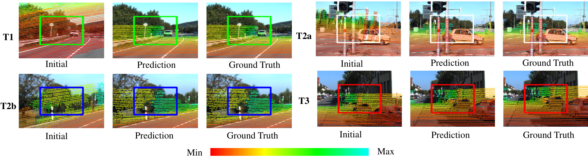
Figure 12: Visualization of online calibration results. This figure presents the online calibration results on the four test sets. The pictures are cropped for better presentation and the areas that can reflect the calibration quality are marked by the bounding boxes. The color bar has the same meaning as Fig. 10.
IV-E Efficiency Evaluation
All-point I2PNet takes 0.048 s per prediction with a 3.38 MB network, compared with 2.984 s for CorrI2P and 0.051 s for the fastest grid-classification baseline. Baseline times include network inference on the RTX 3090 and pose post-processing on a Xeon Gold 6346; I2PNet has no separate pose solver. Its approximately 20 Hz figure is this measured registration runtime, excluding global map retrieval and a complete deployed robot stack.
IV-F Iterations of the Fine Registration
Four fine iterations improve conditional error to 0.77°/0.20 m at 0.069 s, versus 0.83°/0.21 m at 0.048 s for one. More iterations offer little further accuracy improvement and can slightly worsen it; recall reaches 99.43% at six versus 98.67% at one. The default favors speed.
The same registration model is also evaluated as an extrinsic-calibration correction method.
V-A Dataset and Data Pre-processing
KITTI raw scans are transformed by synthetic calibration errors. Training combines 24,000 joint-error examples within ±0.2 m/±15°, 3,000 translation-only examples within ±0.3 m, and 3,000 rotation-only examples within ±20°. Four 2,000-example tests vary drive splits and error ranges; T2a uses the training-drive pool with separately sampled perturbations, whereas T1/T2b use held-out drives. T3 uses another date/drive and ±0.3 m/±2° errors. I2PNet receives no extra T3 fine-tuning, unlike the cited RGGNet comparison. Images resize to 352×1216 and all scan points are used.
Equations 31–32
(31)
(32)
V-B Experiment Result and Visualization
Evaluation uses mean Lie-algebra pose error and mean recalibration rate, a normalized error-reduction measure. I2PNet’s recalibration rates are 99.04%, 98.61%, 97.81%, and 97.21% on T1, T2a, T2b, and T3. These are improvements in synthetic calibration-error metrics, not percentages of perfectly calibrated sensors. The retained overlays show results under all four perturbation regimes.
Equation 33
(33)
VI Conclusion
Joint raw-point/image association and pose regression improve the tested localization and calibration results, with relatively fast inference. The main unresolved issue is scale: fine-grained registration cannot directly search kilometer-scale maps, so the authors propose adding place recognition to select a local map. Further practical dependencies include an accurate map, supplied camera intrinsics, suitable initialization or map pairing, and learned generalization to new sensors and environments. Conditional error reporting and synthetic perturbations bound the interpretation of the reported accuracy.
-A Network Hyperparameters
The complete table specifies feature channels, neighbor counts, sampling strides, kernel sizes, and distance thresholds for every module. The first vertical point stride adapts to 32- or 64-row scans. Coarse correspondence uses all image pixels or 32 neighbors depending on the initial-error regime; fine matching uses 32. These task-dependent settings are part of the reported method.
[1]
P. J. Besl and N. D. McKay, “Method for registration of 3-d shapes,” in
Sensor fusion IV: control paradigms and data structures, vol. 1611,
1992, pp. 586–606.
[2]
J. Yang, H. Li, and Y. Jia, “Go-icp: Solving 3d registration efficiently and
globally optimally,” in Proc. Int. Conf. Comput. Vis., 2013, pp.
1457–1464.
[3]
Z. Liu, S. Zhou, C. Suo, P. Yin, W. Chen, H. Wang, H. Li, and Y.-H. Liu,
“Lpd-net: 3d point cloud learning for large-scale place recognition and
environment analysis,” in Proc. Int. Conf. Comput. Vis., 2019, pp.
2831–2840.
[4]
W. Lu, G. Wan, Y. Zhou, X. Fu, P. Yuan, and S. Song, “Deepvcp: An end-to-end
deep neural network for point cloud registration,” in Proc. Int. Conf.
Comput. Vis., 2019, pp. 12–21.
[5]
Z. J. Yew and G. H. Lee, “Rpm-net: Robust point matching using learned
features,” in Proc. IEEE Conf. Comput. Vis. Pattern Recognit., 2020,
pp. 11 824–11 833.
[8]
Y. Ke and R. Sukthankar, “Pca-sift: A more distinctive representation for
local image descriptors,” in Proc. IEEE Comput. Soc. Conf. Comput.
Vision Pattern Recog., vol. 2, 2004, pp. II–II.
[9]
T. Sattler, B. Leibe, and L. Kobbelt, “Fast image-based localization using
direct 2d-to-3d matching,” in Proc. Int. Conf. Comput. Vis., 2011,
pp. 667–674.
[10]
T. Sattler, B. Leibe, and L. Kobbelt, “Efficient & effective prioritized
matching for large-scale image-based localization,” IEEE Trans.
Pattern Anal. Mach. Intell., vol. 39, no. 9, pp. 1744–1756, 2016.
[12]
R. W. Wolcott and R. M. Eustice, “Visual localization within lidar maps for
automated urban driving,” in Proc. Int. Conf. Intell. Robots
Syst.IEEE, 2014, pp. 176–183.
[13]
G. Pascoe, W. Maddern, and P. Newman, “Direct visual localisation and
calibration for road vehicles in changing city environments,” in Proc.
Int. Conf. Comput. Vis. Workshops, 2015, pp. 9–16.
[14]
T. Caselitz, B. Steder, M. Ruhnke, and W. Burgard, “Monocular camera
localization in 3d lidar maps,” in Proc. Int. Conf. Intell. Robots
Syst., 2016, pp. 1926–1931.
[16]
M. Feng, S. Hu, M. H. Ang, and G. H. Lee, “2d3d-matchnet: Learning to match
keypoints across 2d image and 3d point cloud,” in Proc. IEEE Int.
Conf. Robot. Autom., 2019, pp. 4790–4796.
[17]
B. Wang, C. Chen, Z. Cui, J. Qin, C. X. Lu, Z. Yu, P. Zhao, Z. Dong, F. Zhu,
N. Trigoni et al., “P2-net: Joint description and detection of local
features for pixel and point matching,” in Proc. Int. Conf. Comput.
Vis., 2021, pp. 16 004–16 013.
[18]
S. Ren, Y. Zeng, J. Hou, and X. Chen, “Corri2p: Deep image-to-point cloud
registration via dense correspondence,” IEEE Trans. Circuits Syst.
Video Technol., 2022.
[19]
J. Li and G. H. Lee, “Deepi2p: Image-to-point cloud registration via deep
classification,” in Proc. IEEE Conf. Comput. Vis. Pattern Recognit.,
2021, pp. 15 960–15 969.
[20]
Y. Jeon and S.-W. Seo, “Efghnet: A versatile image-to-point cloud registration
network for extreme outdoor environment,” IEEE Robot. Autom. Lett.,
vol. 7, no. 3, pp. 7511–7517, 2022.
[21]
D. Cattaneo, D. G. Sorrenti, and A. Valada, “Cmrnet++: Map and camera agnostic
monocular visual localization in lidar maps,” arXiv:2004.13795, 2020.
[22]
M. A. Fischler and R. C. Bolles, “Random sample consensus: a paradigm for
model fitting with applications to image analysis and automated
cartography,” Commun. ACM, vol. 24, no. 6, pp. 381–395, 1981.
[23]
Y. I. Abdel-Aziz, H. M. Karara, and M. Hauck, “Direct linear transformation
from comparator coordinates into object space coordinates in close-range
photogrammetry,” Photogramm. Eng. Remote Sens., vol. 81, no. 2, pp.
103–107, 2015.
[24]
V. Lepetit, F. Moreno-Noguer, and P. Fua, “Epnp: An accurate o (n) solution to
the pnp problem,” Int. J. Comput. Vis., vol. 81, no. 2, pp. 155–166,
2009.
[25]
D. W. Marquardt, “An algorithm for least-squares estimation of nonlinear
parameters,” J. Soc. Ind. Appl. Math., vol. 11, no. 2, pp. 431–441,
1963.
[26]
D. Cattaneo, M. Vaghi, A. L. Ballardini, S. Fontana, D. G. Sorrenti, and
W. Burgard, “Cmrnet: Camera to lidar-map registration,” in Proc. IEEE
Intell. Transp. Syst. Conf., 2019, pp. 1283–1289.
[27]
M.-F. Chang, J. Mangelson, M. Kaess, and S. Lucey, “Hypermap: Compressed 3d
map for monocular camera registration,” in Proc. IEEE Int. Conf.
Robot. Autom.IEEE, 2021, pp.
11 739–11 745.
[28]
K. Chen, H. Yu, W. Yang, L. Yu, S. Scherer, and G.-S. Xia, “I2d-loc: Camera
localization via image to lidar depth flow,” ISPRS Journal of
Photogrammetry and Remote Sensing, vol. 194, pp. 209–221, 2022.
[29]
A. Geiger, P. Lenz, C. Stiller, and R. Urtasun, “Vision meets robotics: The
kitti dataset,” Int. J. Robot. Res., vol. 32, no. 11, pp. 1231–1237,
2013.
[30]
H. Caesar, V. Bankiti, A. H. Lang, S. Vora, V. E. Liong, Q. Xu, A. Krishnan,
Y. Pan, G. Baldan, and O. Beijbom, “nuscenes: A multimodal dataset for
autonomous driving,” in Proc. IEEE Conf. Comput. Vis. Pattern
Recognit., 2020, pp. 11 621–11 631.
[31]
J. Yin, A. Li, T. Li, W. Yu, and D. Zou, “M2dgr: A multi-sensor and
multi-scenario slam dataset for ground robots,” IEEE Robot. Autom.
Lett., vol. 7, no. 2, pp. 2266–2273, 2021.
[32]
M.-F. Chang, J. Lambert, P. Sangkloy, J. Singh, S. Bak, A. Hartnett, D. Wang,
P. Carr, S. Lucey, D. Ramanan et al., “Argoverse: 3d tracking and
forecasting with rich maps,” in Proc. IEEE Conf. Comput. Vis. Pattern
Recognit., 2019, pp. 8748–8757.
[33]
P. Sun, H. Kretzschmar, X. Dotiwalla, A. Chouard, V. Patnaik, P. Tsui, J. Guo,
Y. Zhou, Y. Chai, B. Caine et al., “Scalability in perception for
autonomous driving: Waymo open dataset,” in Proc. IEEE Conf. Comput.
Vis. Pattern Recognit., 2020, pp. 2446–2454.
[34]
J. Houston, G. Zuidhof, L. Bergamini, Y. Ye, L. Chen, A. Jain, S. Omari,
V. Iglovikov, and P. Ondruska, “One thousand and one hours: Self-driving
motion prediction dataset,” in Conference on Robot Learning. PMLR, 2021, pp. 409–418.
[35]
Y. Zhong, “Intrinsic shape signatures: A shape descriptor for 3d object
recognition,” in Proc. Int. Conf. Comput. Vis Workshops, 2009, pp.
689–696.
[36]
D. Sun, X. Yang, M.-Y. Liu, and J. Kautz, “Pwc-net: Cnns for optical flow
using pyramid, warping, and cost volume,” in Proc. IEEE Conf. Comput.
Vis. Pattern Recognit., 2018, pp. 8934–8943.
[37]
W. Wu, Z. Y. Wang, Z. Li, W. Liu, and L. Fuxin, “Pointpwc-net: Cost volume on
point clouds for (self-) supervised scene flow estimation,” in Proc.
Eur. Conf. Comput. Vis., 2020, pp. 88–107.
[38]
G. Wang, X. Wu, Z. Liu, and H. Wang, “Hierarchical attention learning of scene
flow in 3d point clouds,” IEEE Transactions on Image Processing,
vol. 30, pp. 5168–5181, 2021.
[39]
G. Wang, Y. Hu, Z. Liu, Y. Zhou, M. Tomizuka, W. Zhan, and H. Wang, “What
matters for 3d scene flow network,” in Proc. Eur. Conf. Comput. Vis.,
2022, pp. 38–55.
[40]
G. Wang, X. Wu, Z. Liu, and H. Wang, “Pwclo-net: Deep lidar odometry in 3d
point clouds using hierarchical embedding mask optimization,” in Proc.
IEEE Conf. Comput. Vis. Pattern Recognit., 2021, pp. 15 910–15 919.
[41]
S. Bileschi, “Fully automatic calibration of lidar and video streams from a
vehicle,” in Proc. Int. Conf. Comput. Vis. Workshops. IEEE, 2009, pp. 1457–1464.
[43]
G. Pandey, J. R. McBride, S. Savarese, and R. M. Eustice, “Automatic extrinsic
calibration of vision and lidar by maximizing mutual information,” J.
Field Robot., vol. 32, no. 5, pp. 696–722, 2015.
[44]
N. Schneider, F. Piewak, C. Stiller, and U. Franke, “Regnet: Multimodal sensor
registration using deep neural networks,” in IEEE Intell. Veh. Symp.
Proc., 2017, pp. 1803–1810.
[46]
G. Iyer, R. K. Ram, J. K. Murthy, and K. M. Krishna, “Calibnet: Geometrically
supervised extrinsic calibration using 3d spatial transformer networks,” in
Proc. Int. Conf. Intell. Robots Syst., 2018, pp. 1110–1117.
[47]
K. Yuan, Z. Guo, and Z. J. Wang, “Rggnet: Tolerance aware lidar-camera online
calibration with geometric deep learning and generative model,” IEEE
Robot. Autom. Lett., vol. 5, no. 4, pp. 6956–6963, 2020.
[48]
C. R. Qi, L. Yi, H. Su, and L. J. Guibas, “Pointnet++: Deep hierarchical
feature learning on point sets in a metric space,” in Proc. Adv.
Neural Inf. Process. Syst., 2017, pp. 5099–5108.
[49]
C. R. Qi, H. Su, K. Mo, and L. J. Guibas, “Pointnet: Deep learning on point
sets for 3d classification and segmentation,” in Proc. IEEE Conf.
Comput. Vis. Pattern Recognit., 2017, pp. 652–660.
[51]
B. Wu, A. Wan, X. Yue, and K. Keutzer, “Squeezeseg: Convolutional neural nets
with recurrent crf for real-time road-object segmentation from 3d lidar point
cloud,” in Proc. IEEE Int. Conf. Robot. Autom., 2018, pp. 1887–1893.
[52]
Q. Hu, B. Yang, L. Xie, S. Rosa, Y. Guo, Z. Wang, N. Trigoni, and A. Markham,
“Randla-net: Efficient semantic segmentation of large-scale point clouds,”
in Proc. IEEE Conf. Comput. Vis. Pattern Recognit., 2020, pp.
11 108–11 117.
[53]
Q. Li, S. Chen, C. Wang, X. Li, C. Wen, M. Cheng, and J. Li, “Lo-net: Deep
real-time lidar odometry,” in Proc. IEEE Conf. Comput. Vis. Pattern
Recognit., 2019, pp. 8473–8482.
[54]
A. Paszke, S. Gross, F. Massa, A. Lerer, J. Bradbury, G. Chanan, T. Killeen,
Z. Lin, N. Gimelshein, L. Antiga et al., “Pytorch: An imperative
style, high-performance deep learning library,” Proc. Adv. Neural Inf.
Process. Syst., vol. 32, pp. 8026–8037, 2019.
[56]
G. Elbaz, T. Avraham, and A. Fischer, “3d point cloud registration for
localization using a deep neural network auto-encoder,” in Proc. IEEE
Conf. Comput. Vis. Pattern Recognit., 2017, pp. 4631–4640.
[57]
Z. J. Yew and G. H. Lee, “3dfeat-net: Weakly supervised local 3d features for
point cloud registration,” in Proc. Eur. Conf. Comput. Vis., 2018,
pp. 607–623.
[58]
J. Li and G. H. Lee, “Usip: Unsupervised stable interest point detection from
3d point clouds,” in Proc. Int. Conf. Comput. Vis., 2019, pp.
361–370.
[59]
X. Bai, Z. Luo, L. Zhou, H. Fu, L. Quan, and C.-L. Tai, “D3feat: Joint
learning of dense detection and description of 3d local features,” in
Proc. IEEE Conf. Comput. Vis. Pattern Recognit., 2020, pp. 6359–6367.
[60]
S. Huang, Z. Gojcic, M. Usvyatsov, A. Wieser, and K. Schindler, “Predator:
Registration of 3d point clouds with low overlap,” in Proc. IEEE Conf.
Comput. Vis. Pattern Recognit., 2021, pp. 4267–4276.
[61]
Y. Ma, Y. Guo, J. Zhao, M. Lu, J. Zhang, and J. Wan, “Fast and accurate
registration of structured point clouds with small overlaps,” in Proc.
IEEE Conf. Comput. Vis. Pattern Recognit., 2016, pp. 1–9.
[62]
Z. Taylor and J. Nieto, “Motion-based calibration of multimodal sensor
extrinsics and timing offset estimation,” IEEE Trans. Robot.,
vol. 32, no. 5, pp. 1215–1229, 2016.
[63]
D. Cattaneo, M. Vaghi, S. Fontana, A. L. Ballardini, and D. G. Sorrenti,
“Global visual localization in lidar-maps through shared 2d-3d embedding
space,” in Proc. IEEE Int. Conf. Robot. Autom., 2020, pp. 4365–4371.
[64]
S. Zheng, Y. Li, Z. Yu, B. Yu, S.-Y. Cao, M. Wang, J. Xu, R. Ai, W. Gu, L. Luo
et al., “I2p-rec: Recognizing images on large-scale point cloud maps
through bird’s eye view projections,” in Proc. Int. Conf. Intell.
Robots Syst.IEEE, 2023, pp.
1395–1400.
[65]
S. Shubodh, M. Omama, H. Zaidi, U. S. Parihar, and M. Krishna, “Lip-loc: Lidar
image pretraining for cross-modal localization,” in Proc. IEEE Winter
Conf. Appl. Comput. Vis. Workshops, 2024, pp. 948–957.