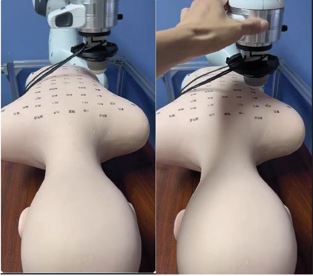
This framework learns position-dependent stiffness from measured motion and interaction force, then uses Lyapunov-based conditions to regulate variable impedance. A symmetry-aware least-squares estimator can also estimate an unknown constant damping parameter. Simulations compare accuracy and speed, and a Franka robot reproduces a massage motion on a silicone dummy. This edition follows the revised manuscript, which uses the Lyapunov formulation and includes hardware experiments.
I Introduction
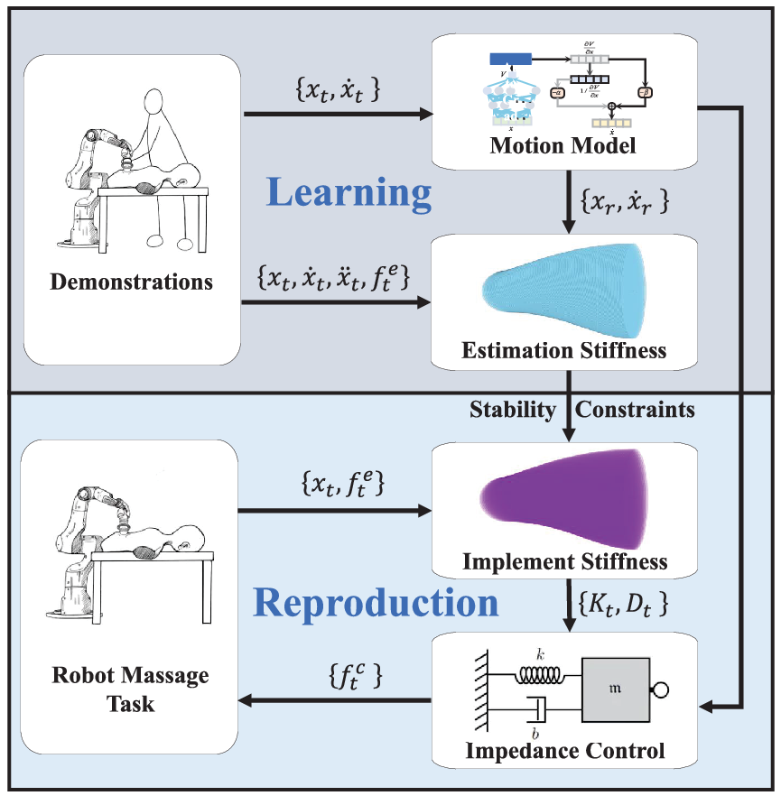
Copying a trajectory does not fully specify contact behavior: the robot also needs suitable compliance. The proposed pipeline estimates full stiffness matrices, learns how they vary with position, and checks conditions governing their use in an impedance controller. The contributions concern estimation, a tractable stability condition, and a demonstrated contact task.
Fig. 1: The framework involves learning variable stiffness from demonstrations and implementing variable impedance control on the Franka robot to perform a massage task.
II RELATED WORK
Prior approaches obtain impedance from force–motion data, muscle signals, manually designed rules, or reinforcement learning. Changing stiffness can inject energy even when every instantaneous stiffness matrix is positive definite. Passivity-based methods address that energy flow through storage functions or virtual energy tanks. The revised paper develops a Lyapunov-based alternative and compares it with an earlier variable-impedance condition.
III Proposed Approach
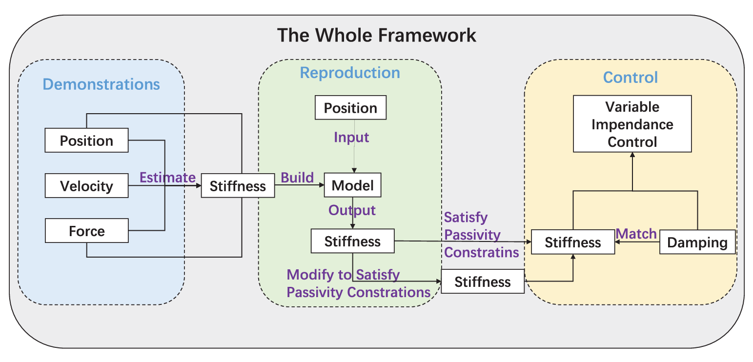
The method models interaction as a virtual mass–spring–damper, estimates its parameters from demonstrations, regresses a state-dependent stiffness profile, and imposes conditions for stable reproduction.
Fig. 2: The process for extracting variable stiffness parameters from demonstration data, followed by the application of these parameters in the implementation of variable impedance control, ensuring the system maintains passivity.
III-A Interaction Model
The end effector is modeled with a constant positive-definite virtual inertia. Position and velocity errors relative to a reference trajectory, measured external force, stiffness, and damping define the desired impedance relation. A slow-motion approximation simplifies the reference-acceleration term for estimation. These assumptions describe the task-space model, not an identification of every physical robot dynamic.
Equations 1–4
(1)
(2)
(3)
(4)
III-B Stiffness Estimation from Demonstrations
A short sliding window treats stiffness as locally constant. Ordinary least squares estimates a full matrix and projects it to the nearest symmetric positive matrix. The proposed estimator instead expands stiffness in a symmetric basis, reducing the unknown coefficients from N² to N(N+1)/2 before the positivity correction.
With unknown constant scalar damping, the damping coefficient joins those unknowns. In the evaluated two-pass procedure, windowwise estimates determine an average damping value, then stiffness is refitted using that value. When damping is constrained to vary with stiffness through the specified eigenvalue relationship, the nonlinear coupling requires a different optimization; the paper uses CMA-ES. Neither case identifies arbitrary independent time-varying damping from unrestricted data.
Equations 5–13
(5)
(6)
(7)
(8)
(9)
(10)
(11)
(12)
(13)
III-C Stiffness Learning and Reproduction
The estimated stiffness is factorized, and Gaussian-kernel ridge regression maps position to the factor’s vectorized entries. Reassembling the matrix as LᵀL enforces positive semidefiniteness; strict positive definiteness additionally requires a nonsingular factor. This permits training from one or several demonstrations.
The reproduced stiffness shapes the task-space control force, which is mapped to joint torques with the Jacobian transpose. Learning a plausible stiffness profile alone does not guarantee stable execution; the following inequalities constrain its use together with damping and virtual inertia.
Equations 14–20
(14)
(15)
(16)
(17)
(18)
(19)
(20)
III-D Novel Lyapunov Functions
The first proposed storage function combines a shifted velocity error with stiffness-weighted position error. Sufficient matrix inequalities involve stiffness, its time derivative, damping, inertia, and a fixed positive parameter α. Unlike the comparison condition, this construction avoids the damping derivative. For the specified scalar critically damped case, the paper derives a less restrictive bound on stiffness variation.
A second storage function uses an inertia-scaled shift and an auxiliary positive-definite matrix. Its conditions retain damping-derivative terms and are compared with the earlier formulation in several dimensions. All displayed inequalities are preserved below.
The stated dissipation supply pairs external force with a shifted error output, ė + αe (or its inertia-scaled version). This is the port used by the paper’s passivity argument. It should not be silently equated with an unconditional physical force–velocity passivity guarantee for arbitrary reference motion, robot dynamics, or environment.
Equations 21–31
(21)
(22)
(23)
(24)
(25)
(26)
(27)
(28)
(29)
(30)
(31)
IV Experiment Results and Discussions
The study includes synthetic parameter-identification tests, a scalar stability comparison, and a contact experiment on a Franka Emika robot. Simulations use MATLAB; the robot implementation uses C++.
IV-A Simulation of Estimating Stiffness
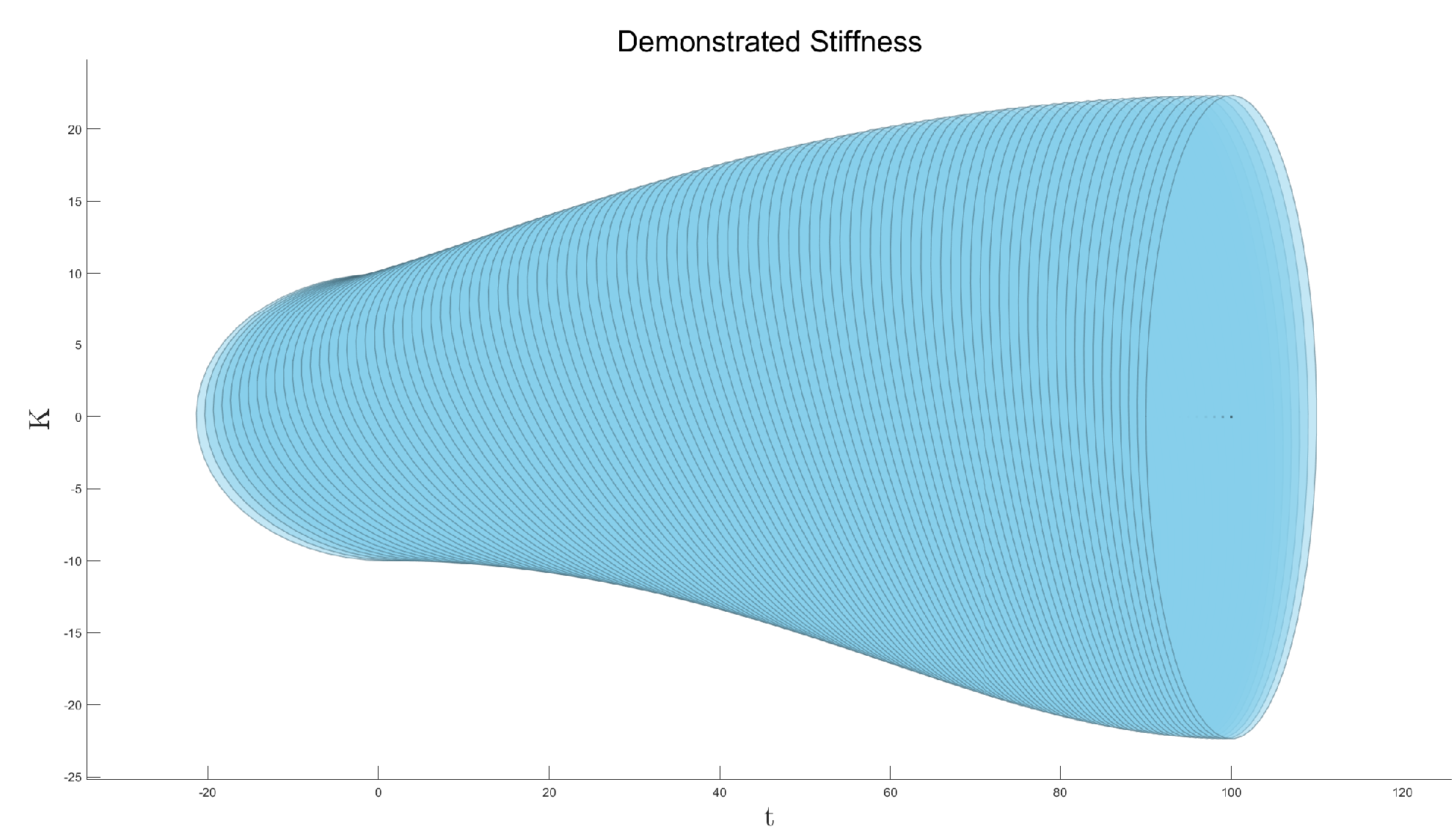
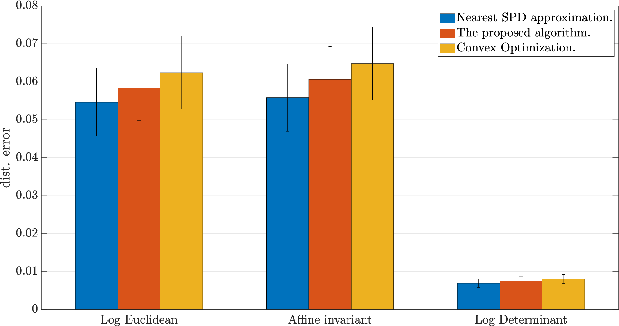
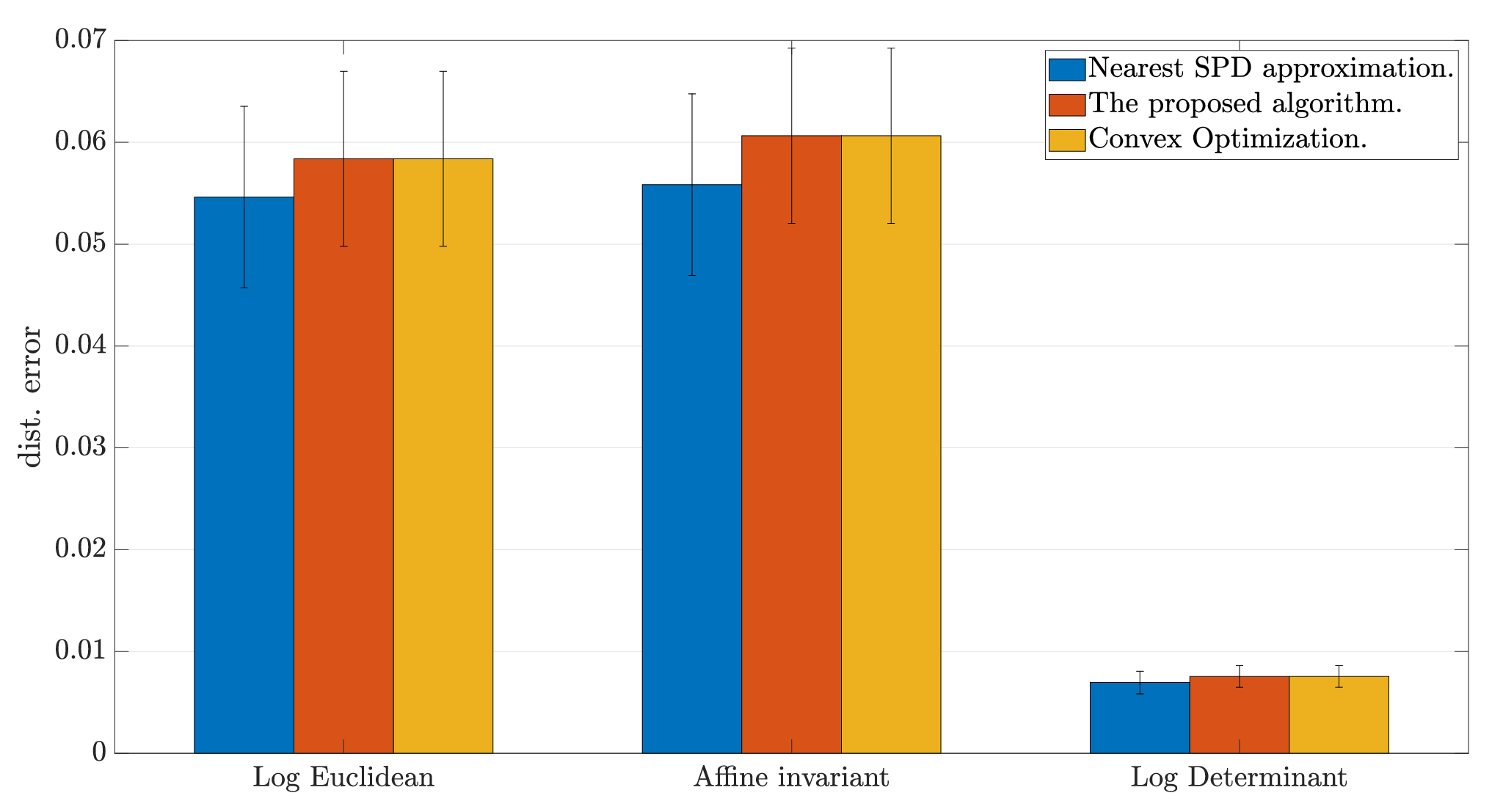
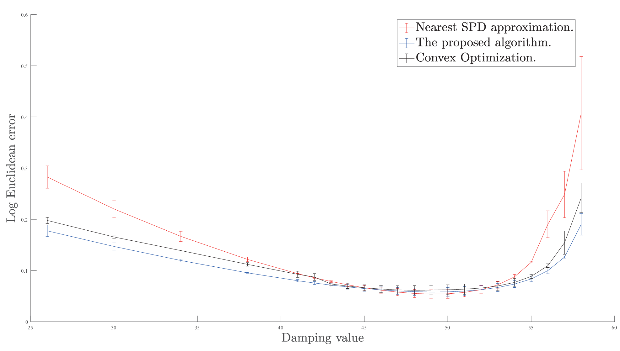
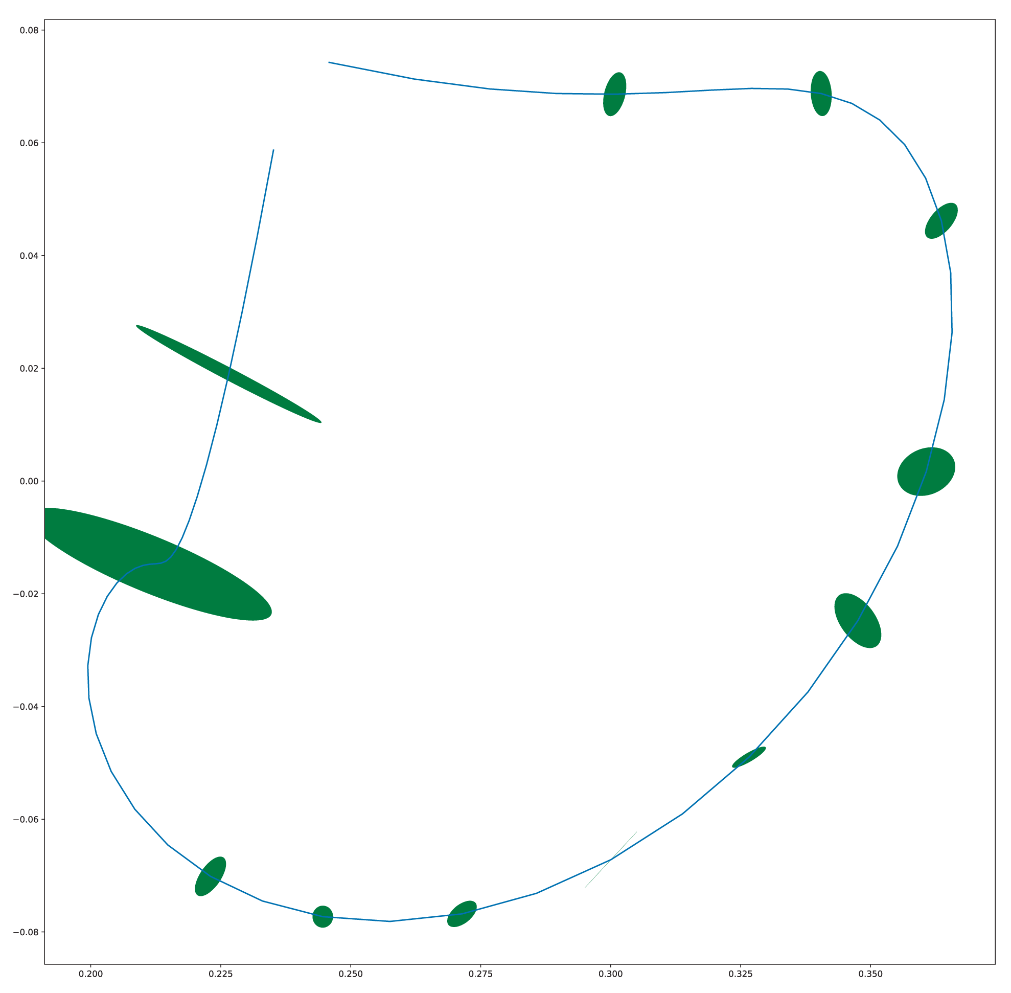
Ten synthetic trajectories use a two-dimensional mass–spring–damper with a rotating stiffness ellipse. A three-sample sliding window estimates stiffness, evaluated with affine-invariant, log-Euclidean, and log-determinant matrix distances. With known damping, nearest-SPD projection is slightly more accurate in the reported case, while the proposed estimator is less sensitive to damping misspecification.
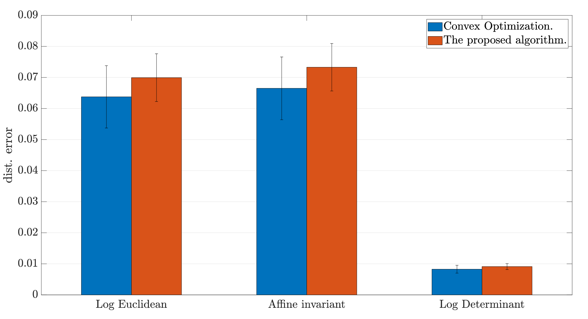
Reported per-step times are 0.23 ms for nearest-SPD estimation, 312 ms for convex optimization, and 0.24 ms for the proposed estimator. Changing the convex objective to match the least-squares normal-equation form closely aligns its estimates with the proposed method. With unknown constant damping, the two-pass estimation remains effective; convex optimization has an accuracy advantage in that example but is much slower.
Fig. 3: The demonstrated stiffness ellipsoids are visualized at different time steps.Equation 32
(32)
Fig. 4: Considering a known constant damping, compare the performance of the estimated stiffness using the proposed algorithm with nearest-SPD approximation and the convex optimization.Equation 33
(33)
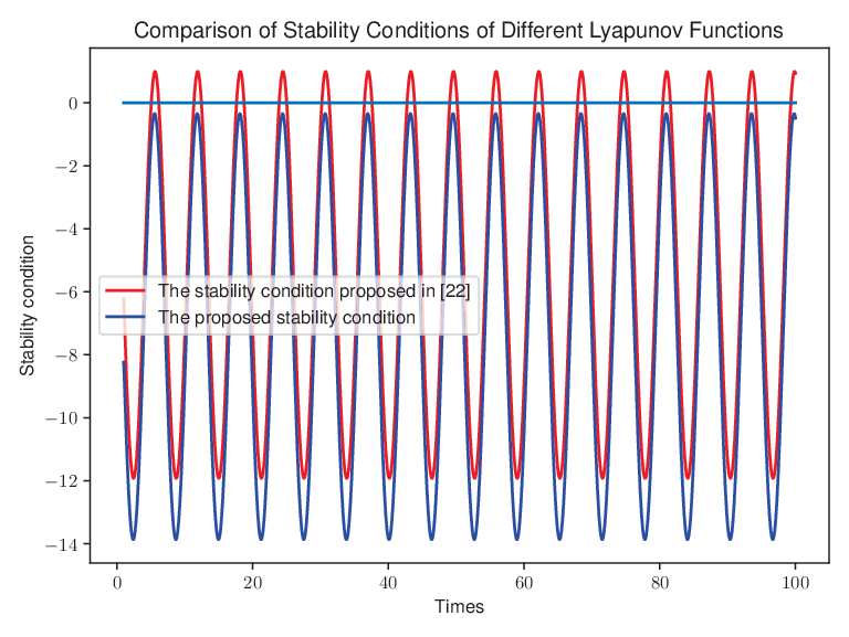
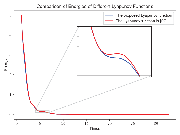
Fig. 5: With known constant damping, compare the performance of the estimated stiffness using the proposed algorithm with nearest-SPD approximation to that using convex optimization to solve the modified objective function.Fig. 6: The stiffness estimation results obtained from applying the proposed algorithm with nearest-SPD approximation and the convex optimization method while varying the damping. Fig. 7: Compare the performance of the estimated stiffness using the proposed algorithm with the convex optimization when assuming that damping is an unknown constant.Fig. 8: Compare the stability condition of the proposed Lyapunov function with the condition presented in [22].Fig. 9: Compare the energy variation of the proposed Lyapunov function with the performance described in [22].Fig. 10:
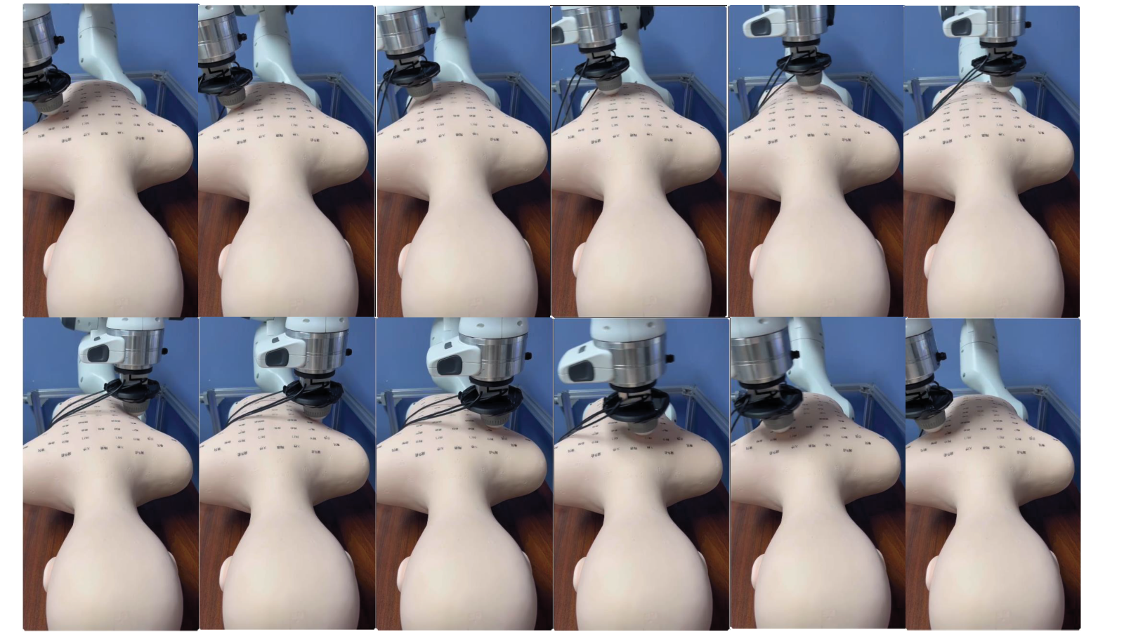
Snapshots of the variable impedance control execution with the Franka Emika robot in the three-dimensional Cartesian space are presented. The robot performs a massage task on a silicone dummy, whose back is not planar. By utilizing the learned stiffness, the robot successfully completes the task.
IV-B Simulation for Validating the Novel Lyapunov Function
A one-dimensional oscillator uses sinusoidally varying desired stiffness and damping tied to its square root. In the chosen parameter setting, the proposed sufficient condition holds while the earlier comparison condition is violated at some times. The plotted storage decreases monotonically. This demonstrates a useful less-conservative case, not universal superiority for all variable-impedance systems.
Equations 34–35
(34)
(35)
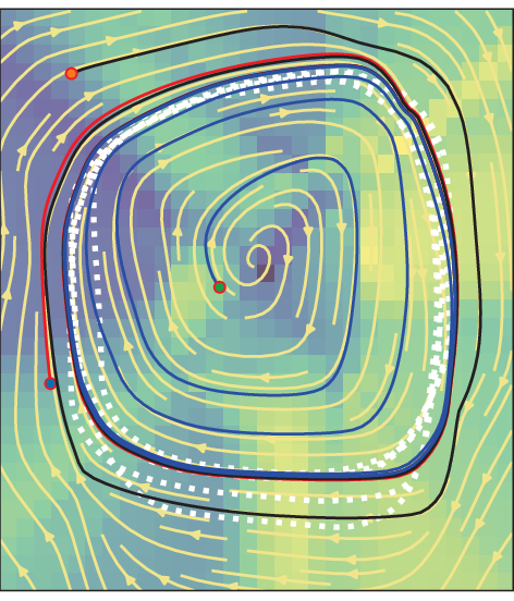
Fig. 11: The limit cycle is learned from the demonstration, with the white dotted line representing the demonstration trajectory. The black, red, and blue lines indicate trajectories that start from different random points and converge to the limit cycle.Fig. 12: The estimated stiffness is based on a segment of the demonstration trajectory, visualized using a stiffness ellipsoid.Fig. 13: Snapshots illustrate the deficiencies of using high and low stiffness for the massage task. With high stiffness (shown on the left), the massage ball may fail to conform to the surface of the silicone dummy, leading to ineffective massage. Conversely, with low stiffness (shown on the right), the robot may become trapped and require additional force to disengage, making it unsuitable for the massage task.
IV-C Validating the Robustness of the Proposed Algorithm in Robot Massage Experiments
A human guides the Franka through a massage motion on a fixed silicone dummy while motion and force are recorded. A learned limit cycle supplies reference motion, and position determines the learned stiffness. A vertical PID force-control component handles contact; damping is adjusted when the stated passivity test is not met.
High constant stiffness can lose conformity to the curved surface, while low stiffness can leave the tool trapped in a low region. The learned varying stiffness reproduces the demonstrated task more effectively in the shown trials. The same dummy and back surface are used for training and reproduction; no human-subject validation or broad quantitative generalization study is reported.
V Conclusions and Future Work
Symmetry-aware estimation and state-dependent stiffness learning offer a fast route from force–motion demonstrations to variable impedance. The practical demonstration is confined to a fixed dummy, and the theoretical conditions rely on the stated model and supply rate. Changing endpoint poses and experiments with human subjects are proposed as future work.
31 references
[1] Y. Zimmermann, J. Song, C. Deguelle, J. Laderach, L. Zhou, M. Hutter, R. Riener, and P. Wolf, ”Human–Robot Attachment System for Exoskeletons: Design and Performance Analysis,” IEEE Transactions on Robotics, vol. 39, no. 4, pp. 3087-3105, 2023.
[2]
A.C. Dometios and C.S. Tzafestas, ”Interaction Control of a Robotic Manipulator With the Surface of Deformable Object,” IEEE Transactions on Robotics, vol. 39, no. 2, pp. 1321-1340, 2023.
[3]
H. Ravichandar, A.S. Polydoros, and S. Chernova, ”Recent Advances in Robot Learning from Demonstration,” Annual Review of Control Robotics and Autonomous Systems, vol. 3, no. 1, pp. 297-330, 2020.
[4]
L. Biagiotti, R. Meattini, D. Chiaravalli, G. Palli and C. Melchiorri, ”Robot Programming by Demonstration: Trajectory Learning Enhanced by sEMG-Based User Hand Stiffness Estimation,” IEEE Transactions on Robotics, vol. 39, no. 4, pp. 3259-3278, 2023.
[5]
Y. Zhang, L. Cheng, H. Li and R. Cao, ”Learning Accurate and Stable Point-to-Point Motions: A Dynamic System Approach,” IEEE Robotics and Automation Letters, vol. 7, no. 2, pp. 1510-1517, 2022.
[6]
C. Zeng, Y. Li, J. Guo, Z. Huang, N. Wang and C. Yang, ”A Unified Parametric Representation for Robotic Compliant Skills With Adaptation of Impedance and Force,” IEEE/ASME Transactions on Mechatronics, vol. 27, no. 2, pp. 623-633, 2022.
[7]
T.K. Best, C.G. Welker, E.J. Rouse and R.D. Gregg, ”Data-Driven Variable Impedance Control of a Powered Knee–Ankle Prosthesis for Adaptive Speed and Incline Walking,” IEEE Transactions on Robotics, vol. 39, no. 3, pp. 2151-2169, 2023.
[8]
E. Burdet, R. Osu, D. Franklin, T.E. Milner, and M. Kawato, ”The central nervous system stabilizes unstable dynamics by learning optimal impedance,” Nature, vol. 414, pp. 446–449, 2001.
[9]
C. Yang, G. Ganesh, S. Haddadin, S. Parusel, A. Albu-Schaeffer and E. Burdet, ”Human-Like Adaptation of Force and Impedance in Stable and Unstable Interactions,” IEEE Transactions on Robotics, vol. 27, no. 5, pp. 918-930, 2011.
[10]
Y. Michel, R. Rahal, C. Pacchierotti, P. R. Giordano and D. Lee, ”Bilateral Teleoperation With Adaptive Impedance Control for Contact Tasks,” IEEE Robotics and Automation Letters, vol. 6, no. 3, pp. 5429-5436, 2021.
[11]
Y. Lin, Z. Chen and B. Yao, ”Unified Motion/Force/Impedance Control for Manipulators in Unknown Contact Environments Based on Robust Model-Reaching Approach,” IEEE/ASME Transactions on Mechatronics, vol. 26, no. 4, pp. 1905-1913, 2021.
[12]
R. Martín-Martín, M. A. Lee, R. Gardner, S. Savarese, J. Bohg and A. Garg, ”Variable Impedance Control in End-Effector Space: An Action Space for Reinforcement Learning in Contact-Rich Tasks,” in Proceedings ofIEEE/RSJ International Conference on Intelligent Robots and Systems, Macau, China, 2019, pp. 1010-1017.
[13]
B. Jonas, S. Freek, T. Evangelos, and S. Stefan, ”Learning
variable impedance control,” The International Journal of
Robotics Research, vol. 30, no. 7, pp. 820-833, 2011.
[14]
Y. Zhu, Q. Wu, B. Chen and Z. Zhao, ”Design and Voluntary Control of Variable Stiffness Exoskeleton Based on sEMG Driven Model,” IEEE Robotics and Automation Letters, vol. 7, no. 2, pp. 5787-5794, 2022.
[15]
J. Arnold and H. Lee, ”Variable Impedance Control for pHRI: Impact on Stability, Agility, and Human Effort in Controlling a Wearable Ankle Robot,” IEEE Robotics and Automation Letters, vol. 6, no. 2, pp. 2429-2436, 2021.
[16]
L. Rozo, S. Calinon, D. G. Caldwell, P. Jimenez, and C. Torras, ”Learning physical collaborative robot behaviors from human demonstrations,”
IEEE Transactions on Robotics, vol. 32, no. 3, pp. 513-527, 2016.
[17]
F.J. Abu-Dakka, L. Rozo, and D. Caldwell, ”Force-based variable
impedance learning for robotic manipulation,” Robotics and Autonomous Systems, vol. 109, pp. 156-167, 2018.
[18]
C. Zeng, C. Yang, H. Cheng, Y. Li, and S.L. Dai, ”Simultaneously
encoding movement and sEMG-based stiffness for robotic skill learning,”
IEEE Transactions on Industrial Informatics, vol. 17, no. 2, pp. 1244–1252, 2021.
[19]
Y. Zhao, K. Qian, S. Bo, Z. Zhang, Z. Li, G. Li, A.A. Dehghani-Sanij, and S.Q. Xie, ”Adaptive Cooperative Control Strategy for a Wrist Exoskeleton Using Model-Based Joint Impedance Estimation,” IEEE/ASME Transactions on Mechatronics, vol. 28, no. 2, pp. 748-757, 2023.
[20]
Y. Zhang, L. Cheng, R. Cao, H. Li, and C. Yang, ”A neural network based framework for variable impedance skills learning from demonstrations,” Robotics and Autonomous Systems, vol. 160, 2023.
[21]
M. Bogdanovic, M. Khadiv and L. Righetti, ”Learning Variable Impedance Control for Contact Sensitive Tasks,” IEEE Robotics and Automation Letters, vol. 5, no. 4, pp. 6129-6136, Oct. 2020.
[22]
K. Kronander and A. Billard, ”Stability Considerations for Variable Impedance Control,” IEEE Transactions on Robotics, vol. 32, no. 5, pp. 1298-1305, 2016.
[23]
F. Ferraguti, C. Secchi, and C. Fantuzzi, “A tank-based approach to
impedance control with variable stiffness,” in Proceedings of IEEE International Conference on Robotics and Automation, Karlsruhe, Germany,
2013, pp. 4948-4953.
[24]
F.E. Tosun and V. Patoglu, ”Necessary and sufficient conditions for the
passivity of impedance rendering with velocity-sourced series elastic
actuation,” IEEE Transactions on Robotics, vol. 36, no. 3, pp. 757-772,
2020.
[26]
O. Khatib, ”A unified approach for motion and force control of robot manipulators: The operational space formulation,” IEEE Journal on Robotics and Automation, vol. 3, no. 1, pp. 43-53, 1987.
[27]
J.H. Nicholas ”Computing a nearest symmetric positive semidefinite matrix,” Linear Algebra and its Applications, 103, vol. 103, pp. 103–118, 1988.
[28]
F.A. Mussa-Ivaldi, N. Hogan, and E. Bizzi, ”Neural, mechanical, and geometric factors subserving arm posture in humans,” The Journal of Neuroscience, vol. 5, no. 10, pp. 2732-2743, 1987.
[29]
S. Jayasumana, R. Hartley, M. Salzmann, H. Li, and M. Harandi, ”Kernel methods on riemannian manifolds with gaussian rbf kernels,” IEEE Transactions on Pattern Analysis and Machine Intelligence, vol. 37, no. 12, pp. 2464-2477, 2015.
[30]
S. Jayasumana, R. Hartley, M. Salzmann, H. Li, and M. Harandi, ”Kernel methods on riemannian manifolds with gaussian rbf kernels,” IEEE Transactions on Pattern Analysis and Machine Intelligence, vol. 37, no. 12, pp. 2464-2477, 2015.
[31]
Y. Zhang, H. Zhang, Y. Zou, H. Li, and L. Cheng, ”Stabilizing Dynamic Systems through Neural Network Learning: A
Robust Approach,” arXiv:2309.08849, 2024.