Overview
Abstract
Imagine planning a route without predicting the color of every leaf along the way. This tutorial develops that distinction: learn representations that keep what matters for a prediction, score compatible possibilities with low energy, and use hidden variables to describe uncertainty. It explains energy-based models, the danger of trivial constant representations, and ways to prevent that collapse. JEPA combines these ingredients to predict one representation from another; H-JEPA stacks predictions at different levels of detail and time. The work teaches a proposed route toward autonomous agents. It does not demonstrate a complete agent or establish that probabilistic learning cannot work.
1 Introduction
These lecture notes follow LeCun’s 2022 Les Houches lectures and explain the ideas behind his autonomous-intelligence position paper. Their motivation is the gap between successful task-specific systems and learning that transfers efficiently across new situations. Read them as a conceptual tutorial, with historical examples, rather than a benchmark comparison of modern systems.
2 Towards autonomous machine intelligence
Large neural networks and fast matrix multiplication enabled major advances in perception and language. The authors use these successes to motivate a next question: what additional machinery would allow a system to learn a world model and use it to plan?
2.1 Applications of machine learning today
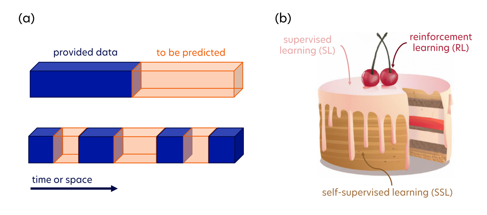
Supervised learning learns from supplied answers; reinforcement learning learns through interactions and rewards. Self-supervised pretraining instead obtains a training signal from relationships inside the observations themselves. The following examples describe applications available when these lectures were prepared.
Transportation
Driver-assistance systems use learned perception for functions such as braking and lane keeping. The paper distinguishes those useful components and geographically restricted robotaxis from the much broader demand of autonomous driving in unfamiliar conditions.
Translation, transcription, accessibility
Translation and speech systems illustrate reusable internal representations: first encode the input, then decode the required output. Multilingual models can share this machinery across many language pairs, including pairs with little direct training data.
Online safety and security
Content moderation combines learned language and visual representations with human review and matching against known material. The historical figures in the paper illustrate deployment at scale; they do not resolve the separate question of who should decide what content is acceptable.
Computer vision
Visual models can identify objects, estimate human pose, and label image pixels. Semantic segmentation assigns a class to each pixel; instance segmentation additionally separates individual objects of the same class.
Medical analysis
The fastMRI example uses learned reconstruction to estimate images from fewer measurements. It illustrates how a network can exploit structure in data. The paper also points toward predicting useful outputs directly from measurements instead of always reconstructing a human-viewable image first.
Biomedical sciences
The examples range from modeling neural activity and gene regulation to predicting protein structure. They show the breadth of learned representations, while remaining distinct scientific tasks rather than evidence of a single general-purpose autonomous system.
Physics
In physics, networks can act as fast approximations to expensive simulations, represent quantum states, or recognize patterns in experimental and astronomical data.
Chemistry and material science
In chemistry and materials research, learned models can help search for compounds, approximate costly calculations, and propose materials with useful properties.
2.2 Limitations of the current machine learning
The authors argue that future agents need three abilities: learn predictive world representations from observation, use those models for deliberate reasoning, and organize long tasks into shorter subplans. Their comparisons with human learning motivate this research program. Broad claims about the limits of language models and the state of applications belong to the 2022–2023 context of the notes.
2.3 New paradigm to autonomous intelligence
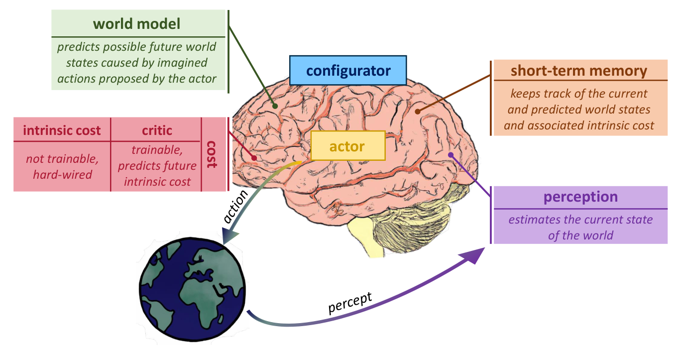
Think of the architecture as a planning loop. Perception estimates the present; a world model predicts candidate futures; an actor searches for actions with low expected cost. An immediate intrinsic cost and a learned critic score those futures, short-term memory supplies recent experience, and a configurator selects the current task. This resembles model predictive control with a learned model. Fully differentiable components are an architectural proposal, not a demonstrated complete implementation.
2.4 Self-supervised learning and representing uncertainty
Predicting a single exact future is difficult because several outcomes may be possible. A pixelwise squared-error predictor can average them into a blurry result. The proposed alternative is to retain predictable, useful information in a representation and represent remaining uncertainty separately. Avoiding explicit normalization can remove one expensive computation; it does not make high-dimensional inference or learning automatically easy.
2.5 Structure of the manuscript
The tutorial first defines energy and latent variables, then explains training and collapse. Classical models provide concrete examples before the final sections assemble the ingredients into JEPA and H-JEPA.
3 Introduction to energy-based models
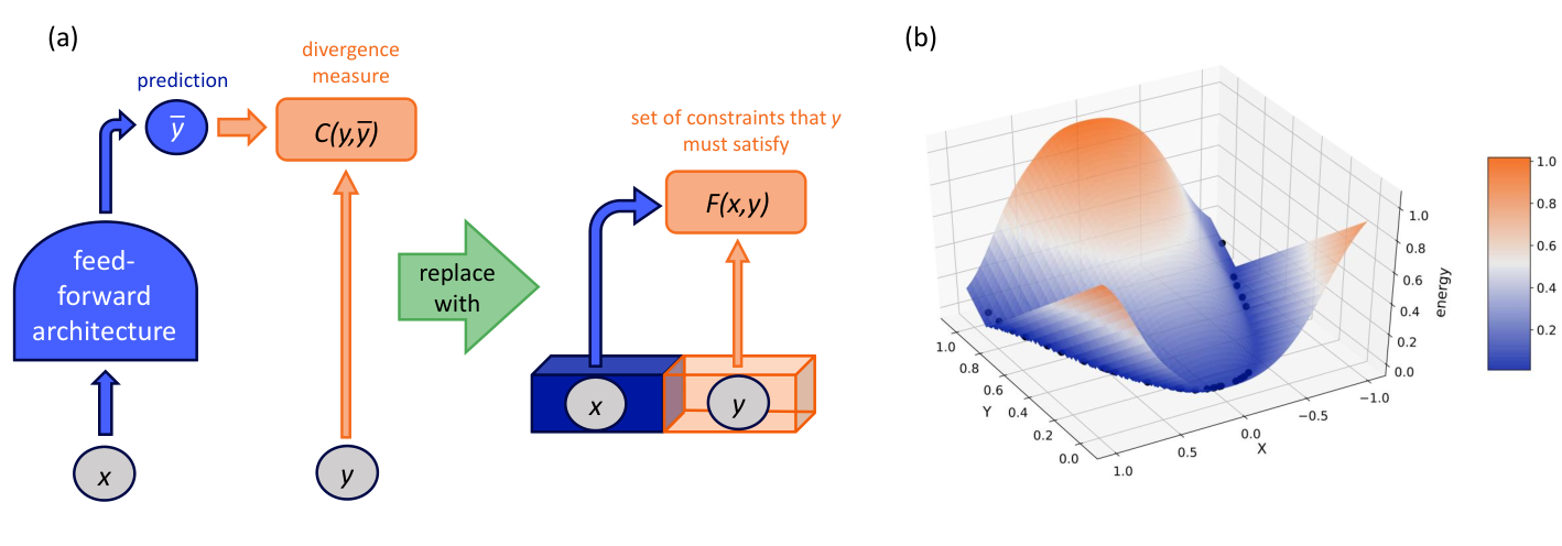
An energy function is a compatibility score: lower means that an input and a candidate answer fit together better. Inference searches for a low-energy answer while keeping the input fixed. Training is a different optimization problem: change the model’s parameters so observed relationships receive useful scores. Multiple low-energy answers can express several compatible outcomes.
3.1 Energy-based models vs. probabilistic models
An energy model can rank answers without assigning probabilities that sum to one. To turn its energies into probabilities, exponentiate negative energy and divide by a partition function that sums or integrates over all answers. That denominator can be costly. Unnormalized scores provide flexibility, but their scales are not automatically comparable across models and their uncertainty is not calibrated. These are tradeoffs; intractability depends on the model and inference method.
Equations 1–2
| (1) |
| (2) |
3.2 Latent variable energy-based models
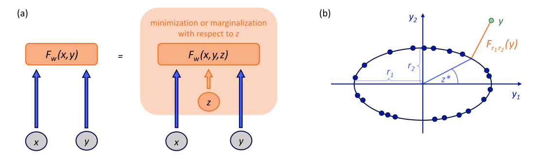
A latent variable describes an unobserved factor, such as an object’s pose or another driver’s possible behavior. For the ellipse example, the latent angle selects a point on the curve. Minimizing over angles finds the closest point; marginalizing combines contributions from all angles. Limiting latent capacity matters: otherwise the latent variable can carry the entire answer and let the model ignore its input. In the source prose, an argmin is sometimes written where an energy value would require a min; the distinction is the optimizing angle versus the resulting score.
| Prediction problem | Examples of latent variables | |||||
|---|---|---|---|---|---|---|
| Face recognition |
| |||||
|
| |||||
| Speech tagging | sentence segmentation into syntactic units, the parse tree | |||||
| Speech recognition | sentence segmentation into phonemes or phones | |||||
| Handwriting recognition | the segmentation of the line into characters |
4 Training an energy-based model
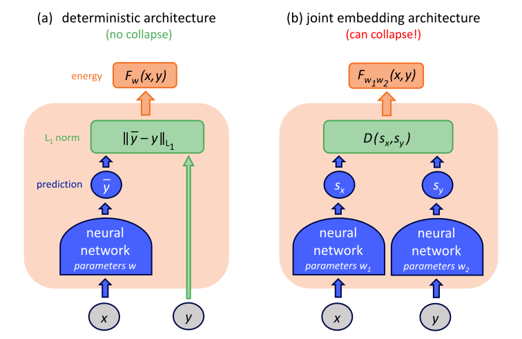
Simply reducing the mismatch of observed pairs can have a useless shortcut: both encoders output the same constant, so every pair appears compatible. A generous latent code can create a similar shortcut by memorizing the answer. The training problem must therefore make correct pairs fit while limiting the set of other inputs that also receive low energy. The following sections present alternative ways of doing this.
4.1 Contrastive methods
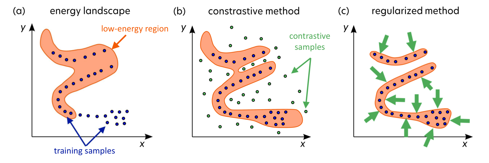
Contrastive learning supplies incompatible alternatives as well as compatible pairs. A hinge loss requires the real pair to beat a negative pair by a margin. The margin prevents a constant energy function from satisfying the objective. Batch-based objectives such as InfoNCE compare a larger group of alternatives.
Equation 3
| (3) |
4.1.1 How to generate contrastive points
Negative examples may be enumerated, sampled, selected because the model currently confuses them, or generated by another network. In a Siamese model, views of different objects can supply negatives. The challenge is finding informative alternatives without spending excessive compute searching a huge output space.
4.1.2 Maximum likelihood as a special case of a contrastive method
For a Gibbs model, the likelihood gradient has two effects: lower the energy of observed data and raise energy in regions the current model favors. The second part can be estimated using samples from that model. Sampling and regularization can be demanding, especially in high dimensions; the discussion motivates alternatives rather than proving that every likelihood-based model must fail.
Equations 4–5
| (4) |
| (5) |
4.2 Architectural and regularized methods
Another strategy limits how much of the input space can receive low energy. A small bottleneck, a finite set of codes, sparsity, or controlled noise can restrict reconstruction capacity. Regularizers can enforce related constraints. The point is to remove the all-inputs-fit shortcut without explicitly generating many negatives.
4.2.1 Regularized autoencoders
Autoencoding compresses an input and reconstructs it. Principal component analysis restricts the representation to a low-dimensional linear space; a bottleneck autoencoder permits a nonlinear space; k-means permits only a finite collection of prototypes; sparse coding discourages using many code components at once. All balance fitting the data against the capacity available to explain it.
Equation
4.2.2 Regularization through the variational marginalization of a latent variable
A stochastic latent code can be regularized by comparing its input-dependent distribution with a reference distribution using KL divergence. If the two stay close, the code cannot freely transmit every detail of the answer. The expected reconstruction energy rewards a useful code, while the information constraint prevents unrestricted memorization.
Equation
5 Examples of energy-based models
Hopfield networks, Boltzmann machines and denoising autoencoders show how an energy interpretation applies to familiar models. Their different training rules make the contrast between fitting observations and controlling unwanted low-energy states concrete.
5.1 Hopfield networks
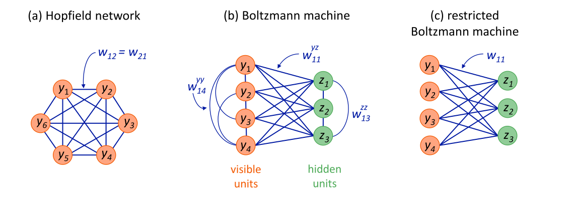
A Hopfield network stores patterns in symmetric connections. Repeatedly updating one neuron according to the others descends toward a locally stable state, which can recover a stored pattern from partial information. A simple Hebbian rule strengthens connections between units active together. Unwanted stable states can also appear, so low energy need not identify a true stored memory.
Equations 6–7
| (6) |
| (7) |
5.2 Boltzmann machines
Boltzmann machines add hidden units and stochastic states. Training compares correlations under observed data with correlations produced by the model: strengthen relationships supported by the data and weaken those the model overproduces. Estimating those model correlations requires sampling, which can be costly. Restricting the connection pattern simplifies some computations without removing every sampling challenge.
Equations 8–12
| (8) |
| (9) |
| (10) |
| (11) |
| (12) | ||||
5.3 Denoising autoencoders
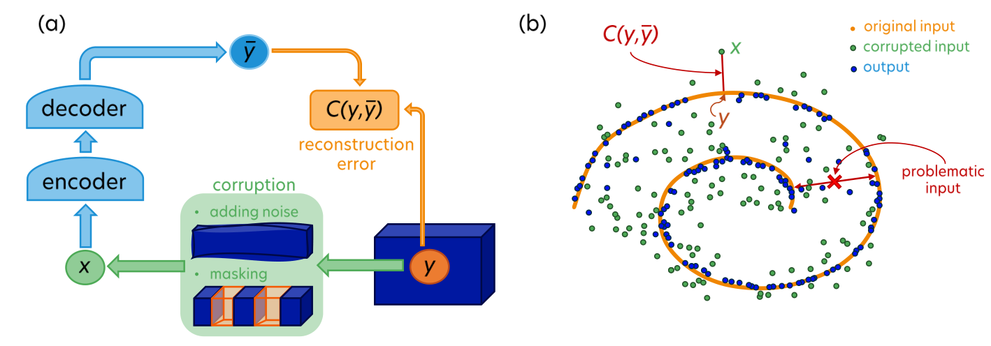
A denoising autoencoder learns to map a corrupted observation back toward clean data. The spiral example makes the goal visible: noisy points should return to the curve. If a point lies equally near two branches, a single deterministic output cannot express both possibilities. Masking creates a related prediction task, while latent variables and representation-space prediction offer ways to handle ambiguity.
6 Building block of proposed autonomous systems of the future
JEPA combines learned representations, prediction and a mechanism for handling uncertainty. Its aim is to compare the information needed for a prediction without requiring a complete reconstruction of the raw observation.
6.1 Joint embedding predictive architecture
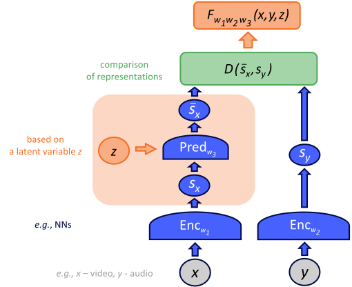
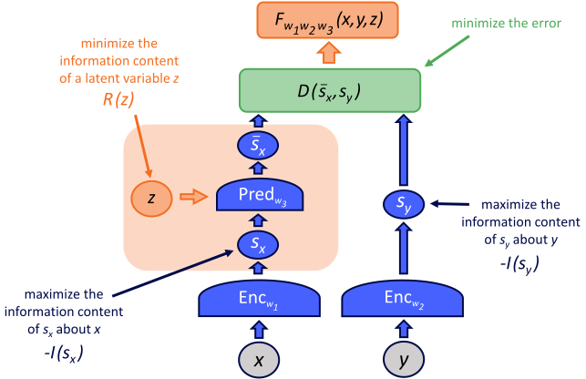
Two encoders map related inputs into representations, and a predictor estimates the target representation using the context and, when needed, a latent variable. Constant outputs must be prevented, and the latent channel must not carry the whole answer. VICReg illustrates explicit regularization: keep each feature’s batch variance above a threshold, reduce cross-feature covariance, and match paired representations. These constraints encourage informative, nonredundant features; decorrelation alone is not a guarantee of statistical independence or complete retained information.
6.2 Hierarchical joint embedding predictive architecture
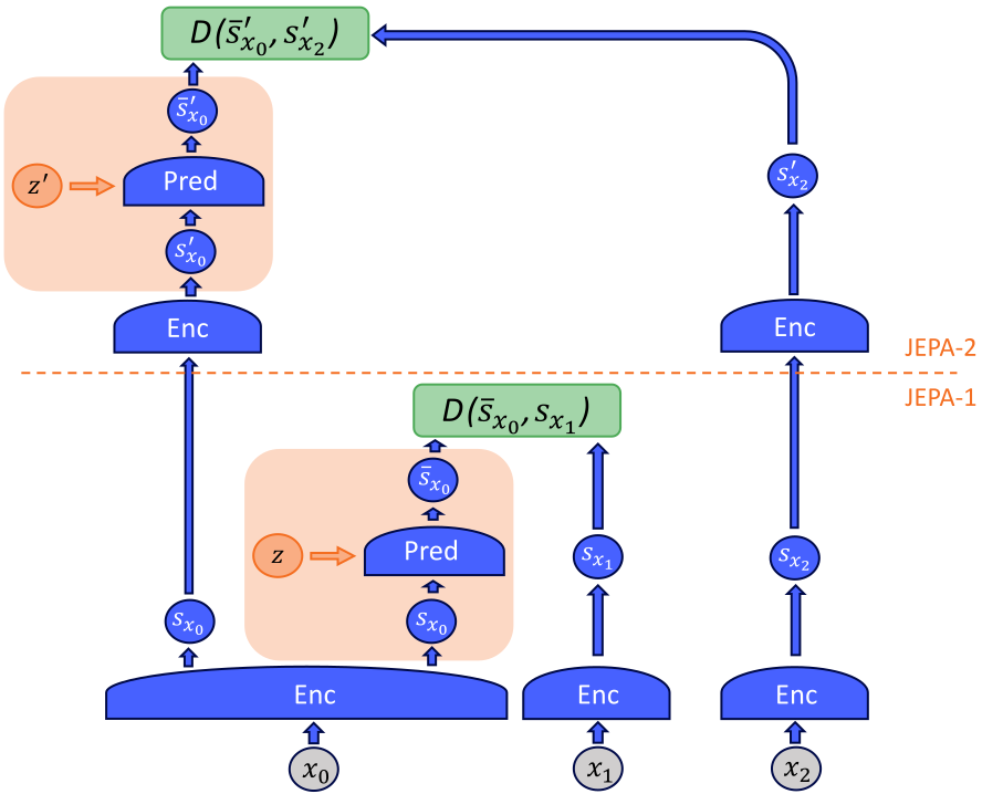
A hierarchy uses detailed representations for short-horizon predictions and more abstract representations for longer horizons. For example, a high level might plan to enter a room while a lower level chooses the next movement. Stacking JEPAs is proposed as a way to learn these levels and support hierarchical planning. The notes present the construction and motivation, rather than an evaluated end-to-end autonomous agent.
7 Conclusion
The tutorial’s main contribution is a connected vocabulary for a research direction: energy scores compatibility, latent variables represent unresolved factors, regularization prevents shortcuts, and JEPA predicts in a learned representation space. H-JEPA adds abstraction and multiple timescales. Which representations, constraints and planning procedures make the full proposal work remains an empirical and algorithmic question.
Acknowledgements
The notes are based on LeCun’s 2022 Les Houches lectures and acknowledge discussions with Alfredo Canziani, Lucas Clarte and Max Daniels.
Funding information
The authors acknowledge support from Polish, Spanish, Catalan and European research programs, including support for the ICFO group. The views expressed are the authors’ own.
List of acronyms
Overview
The source acronym list is retained below; the Terms tab also supplies definitions beside the reading text.
Appendix A How to turn energies into probabilities
The appendix gives the probability dictionary for energy models. A Gibbs distribution converts low energies into high probabilities by exponentiating and normalizing. Conditioning holds an observed variable fixed; marginalizing integrates out a hidden variable. The resulting free energy is a logarithm of a sum or integral of exponentiated energies. Minimization keeps the best latent explanation, whereas marginalization combines all explanations with energy-dependent weights.
Equations A1–A5
| (A1) |
| (A2) |
| (A3) |
| (A4) |
| (A5) |