At a glance
Graphs of Geodesically-Convex Sets (GGCS) extend convex-set motion planning to configuration spaces with periodic angles, including continuous revolute joints and planar mobile bases. On a flat manifold, local distance-preserving coordinates turn region constraints, path costs, and transitions between charts into an ordinary Graph of Convex Sets (GCS) problem.
The construction supports exact mixed-integer optimization or faster convex relaxation and rounding. Practical guarantees apply to the collision-free region cover that has been constructed, and the demonstrated trajectories use approximate rounding. Simulated examples include a toroidal point robot, a planar arm, a modified KUKA iiwa, and a PR2 mobile manipulator.
I Introduction
Sampling planners can struggle to cover high-dimensional configuration spaces, while nonlinear trajectory optimizers can become trapped in poor local solutions. The GCS formulation and GCS motion planner of Marcucci et al. address obstacle-induced nonconvexity by choosing a sequence of convex collision-free regions and optimizing the continuous path within them.
Periodic joints break a naive Euclidean coordinate model: angles differing by a full turn describe the same configuration. GGCS represents that topology with overlapping manifold charts rather than artificial joint limits or duplicated angle ranges. The scope is kinematic planning with suitable convex costs and constraints; nonlinear dynamics, closed kinematic chains, and ball-joint geometry are not handled by this reduction.
II Related Work
Probabilistic roadmaps and rapidly exploring trees offer asymptotic sampling guarantees, but their practical coverage can be costly. Trajectory optimization directly searches a parameterized curve but generally lacks global guarantees in obstacle-rich problems. Mixed-integer methods encode discrete route choices, with convex relaxations and rounding sometimes reducing their cost substantially.
Riemannian motion policies use geometric metrics to combine controllers. Here, geometry instead supplies a global path-planning formulation over a finite collection of local regions. The reduction reuses ordinary GCS solvers when its flatness and convexity assumptions hold.
III Preliminaries
The construction needs coordinate charts, a metric for measuring path length, and a notion of convexity that respects the configuration space’s topology. The original mathematical definitions are retained below.
III-A Riemannian Geometry
A chart maps a local manifold neighborhood to Euclidean coordinates; overlapping charts are connected by transition maps. Tangent vectors represent velocities, and a Riemannian metric supplies their inner products. Integrating speed gives coordinate-independent curve length; distance is the infimum over connecting curve lengths.
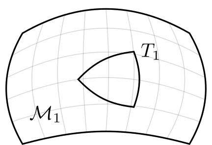
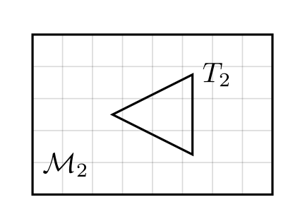
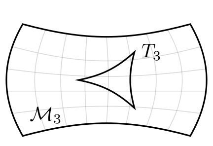
A local isometry preserves the metric. Geodesics are locally length-minimizing constant-speed curves, and the exponential map follows a geodesic from a point in a chosen tangent direction. Curvature measures departure from Euclidean local geometry, illustrated by Figure 2. Flat manifolds have zero sectional curvature, and products of flat manifolds remain flat. The choice of metric is part of this formulation.
Equations 1–2
| (1) |
| (2) |
III-B Convex Analysis on Manifolds
A strongly geodesically convex region contains the unique globally shortest geodesic between any two of its points. This stronger definition ensures that intersections stay geodesically convex and that each segment has an unambiguous shortest realization. Small enough neighborhoods satisfy the condition, with the convexity radius bounding their size.
A geodesically convex function is convex along each geodesic in its domain. The retained inequality is the manifold counterpart of ordinary convexity. These definitions alone do not provide a general-purpose mixed-integer solver on arbitrary curved spaces.
Equations 3–4
| (3) |
| (4) |
IV Problem Statement
The formal problem minimizes Riemannian arc length between two configurations in the closure of a bounded, connected collision-free region. The ambient configuration manifold is assumed connected and complete. The closure permits boundary configurations in the mathematical model; practical collision guarantees depend on the chosen certified regions and collision geometry.
Equation 5
| (5) |
V Graphs of Geodesically-Convex Sets
Each graph vertex carries a geodesically convex region, and each directed edge has a nonnegative geodesically convex cost on the product of its endpoint regions. A discrete route and one continuous choice per visited vertex jointly determine the total cost.
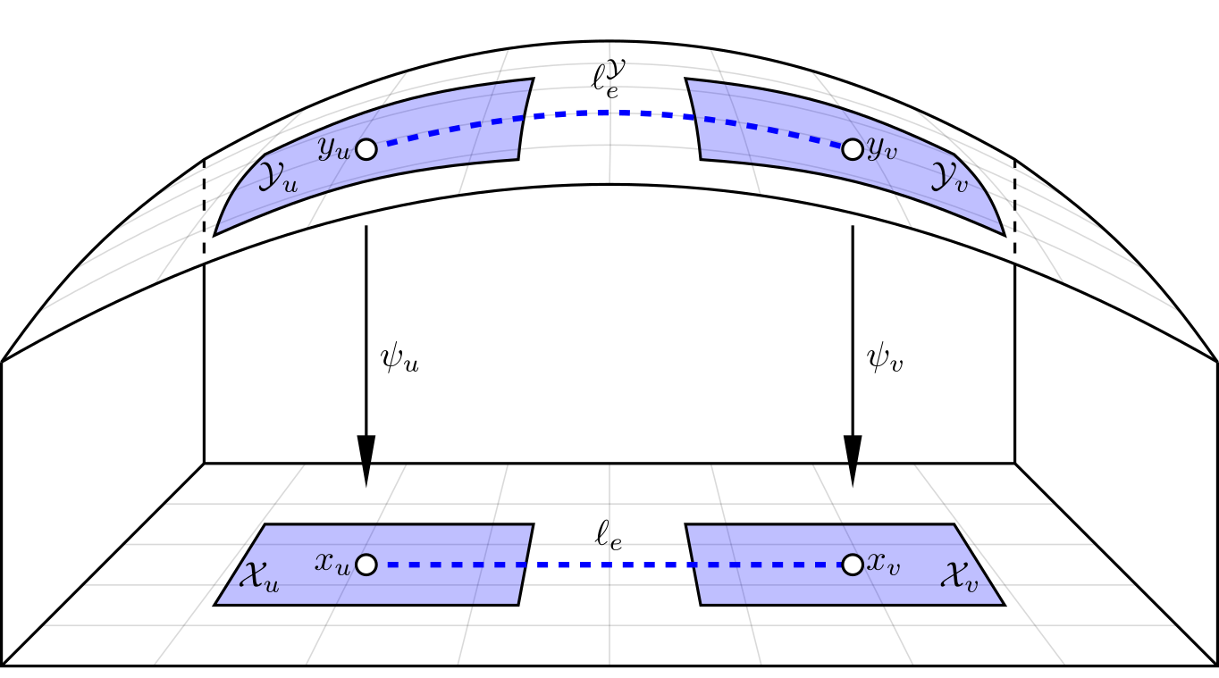
Applying a chart to each region produces a candidate Euclidean GCS problem. That conversion is useful only if the charted regions and transformed costs remain convex. Flat configuration spaces built from one-degree-of-freedom joints and a planar mobile base meet the later assumptions with suitable charts. Universal joints can be modeled as two one-degree-of-freedom joints; the same geometric argument does not extend to ball joints.
Equations 6–7
| (6) |
| (7) |
Equation 8
| (8) |
VI Motion Planning with GGCS
The paper first states existence of a shortest continuous curve, then assumes a finite chart cover whose region closures are strongly geodesically convex and cover the relevant free-space closure. These are substantive conditions, not automatic properties of arbitrary obstacle spaces. The original theorem and assumption statements are retained below.
Theorem 2 replaces the portion between the first and last visit to each region by its unique minimizing geodesic. Under the stated setup, this yields a piecewise-geodesic optimum that visits each region at most once, matching the graph’s simple-path representation. Equation 9 preserves the replacement construction. The appendix’s general existence argument has a completeness gap discussed in Appendix A.1.
Theorem 1.
(Existence of Optimal Trajectories) For any , there exists a continuous curve connecting them such that .
Assumption 1.
We are given a finite atlas of . For each , the closure is g-convex as a subset of . Furthermore, the union of the closures covers .
Theorem 2.
(Piecewise Geodesic Optimal Paths) Let , and suppose the sets satisfy Assumption 1. Then there is a curve connecting them, such that the following are true:
- •
- •
is a piecewise geodesic of
- •
Each geodesic segment is contained in some
- •
passes through each at most once.
Equation 9
| (9) |
VI-A Formulation as a GCS Problem
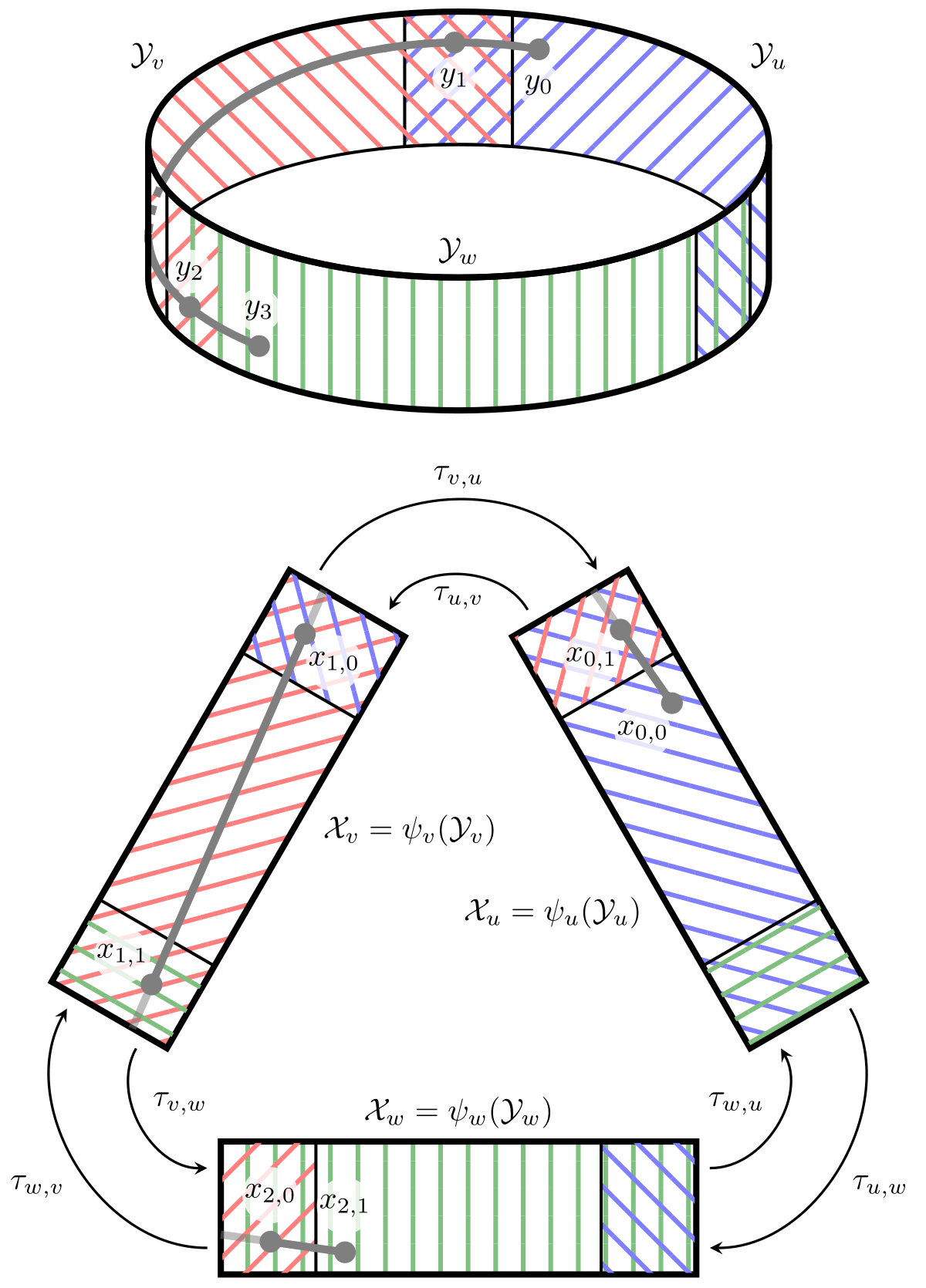
With a flat ambient manifold and locally isometric charts, charted regions are Euclidean convex sets, within-region distances become Euclidean norms, and chart transitions are affine isometries. For the product coordinates used here, transitions can be aligned as translations.
Each graph vertex represents a segment’s two endpoints. Its cost is the segment length; adjacent endpoints agree after applying the transition map. These are convex constraints and costs, so ordinary GCS machinery applies. Figure 4 shows how chart-space segments lift back to the cylinder.
Theorem 3 compares the two constructions in both directions: every feasible GCS path lifts to a feasible piecewise geodesic of equal length, and an optimal curve with Theorem 2’s structure induces a feasible graph solution. Exact global optimality is conditional on this represented region cover and an exact solve; relaxation and randomized rounding are approximate.
Assumption 2.
is flat. Also, each is a local isometry into Euclidean space, viewed as a Riemannian manifold with the canonical Euclidean metric.
Theorem 3.
Equations 10–13
| (10) |
| (11) |
| (12) |
| (13) | ||||
Equations
VI-B Construction of the Atlas
IRIS grows collision-free convex regions around chosen seeds in local Euclidean coordinates. The implementation limits each joint’s region extent using its convexity radius, with a small numerical margin, so periodic coordinates do not admit a shorter route around the other side of the manifold. Theorem 4 states the sufficient product-space condition.
The generated regions provide an inner approximation of free space. Configurations outside that cover are effectively treated as obstacles, so an exact solve optimizes within the covered space rather than necessarily finding the shortest path in the robot’s entire physical free space. Seed choice and connectivity therefore matter.
Theorem 4.
Suppose , where each has a convexity radius . Let be a coordinate chart, with a local isometry and convex in Euclidean space. If is flat and the diameter of is less than , then is g-convex.
VI-C More General Motion Planning
Piecewise Bézier curves permit duration and energy costs, velocity bounds, and continuity requirements beyond position. On flat regions, ordinary segment-local expressions carry over. Matching derivatives across charts uses the transition map’s linear pushforward; aligned product charts make that map the identity. Equation 14 is retained in its original notation.
Equation 14
| (14) |
VI-D Positive Curvature Induces Nonconvexity
Positive sectional curvature obstructs this particular convex-distance reduction. Theorem 5 states that distance on the product manifold is nonconvex in every neighborhood of a point with a positive-curvature tangent plane. This explains the limitation for SO(3), ball joints, and unconstrained spatial rigid-body orientation. It does not say that every planning formulation on those spaces is impossible.
Theorem 5.
Let be a Riemannian manifold, let and such that . Then for any neighborhood containing , is nonconvex on .
VII Experiments
All demonstrations are implemented in Drake. They exercise periodic coordinates, region connectivity, and obstacle-rich high-dimensional planning. The original figure and table links retain access to interactive trajectory recordings.
VII-A Point Robot
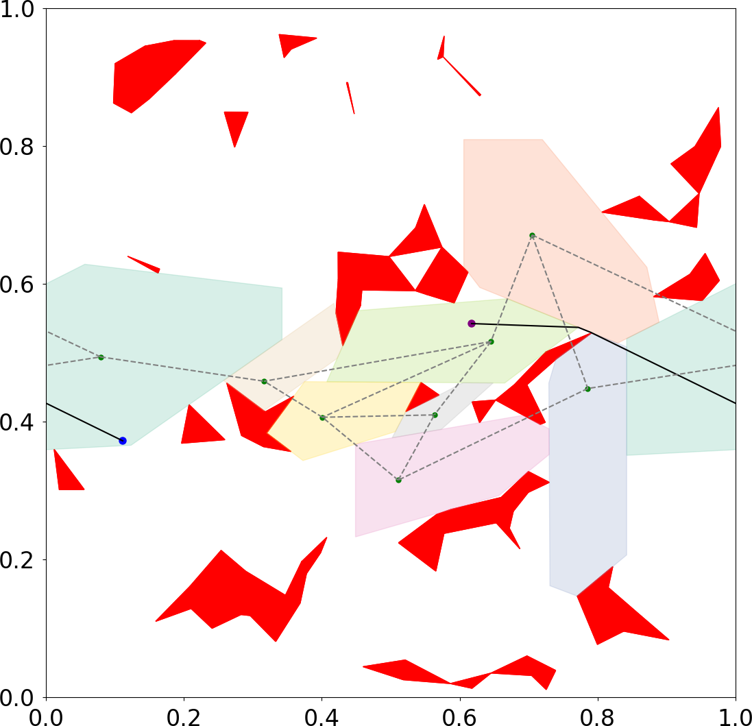
A point robot moves on a two-dimensional torus represented by a unit square with opposite edges identified. Figure 5 shows obstacles, overlapping regions, and a path that wraps around the boundary. Planning took 0.79 seconds in this example.
VII-B Planar Arm
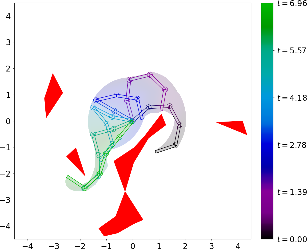
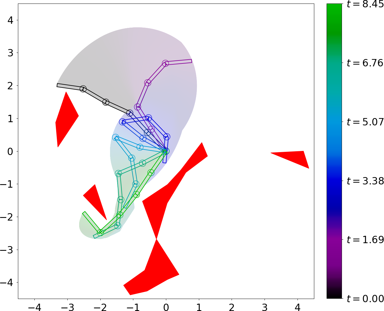
The planar arm has five continuous revolute joints, with self-collision excluded from the model. Figure 6 retains both trajectories and swept collision volumes. They took 5.36 and 4.63 seconds to plan. The second uses more than a full turn of its middle joint, illustrating why a fixed one-turn coordinate interval can exclude a useful solution.
VII-C Modified KUKA iiwa Arm
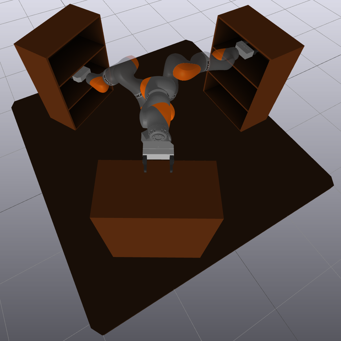
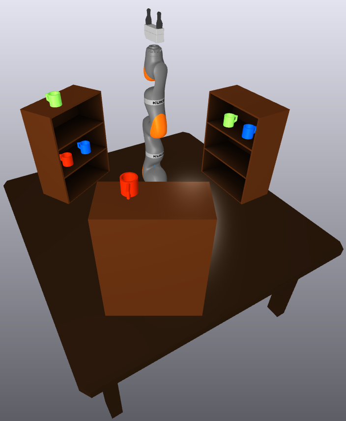
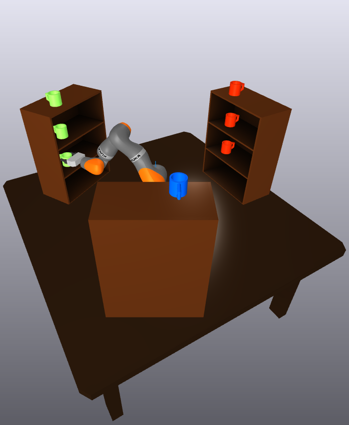
In simulation, the first joint of a seven-joint KUKA iiwa is made continuous. A specified sequence of fourteen motions sorts mugs across shelves; the planner solves each geometric motion rather than choosing the task sequence. Eighteen seed-based regions are refined as mug locations change, including collision checks for a held mug.
Figures 7 and 8 show seed configurations and initial/final states. Mean planning time per motion is 25.75 seconds, ranging from 4.63 to 50.30 seconds. The continuous base joint avoids unnecessary unwinding. Appendix B gives the trajectory and region-generation details.
VII-D PR2 Bimanual Mobile Manipulator
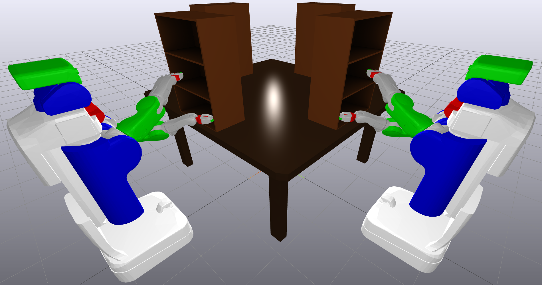
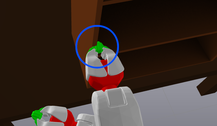
The PR2 experiment plans in a fifteen-dimensional configuration space after fixing wrist/gripper joints. Shelf-reaching and crossed-arm poses seed the regions; additional intermediate seeds are chosen manually to maintain connectivity. Figure 9 shows a resulting trajectory.
Tables I and II preserve every path length, online planning time, collision timestamp, and recording link. GGCS takes about 25.5–66.2 seconds per query, while the prebuilt roadmap answers in roughly half a second but produces much longer paths. Roadmap construction takes 124.39 seconds; parallel generation of the IRIS regions takes 156.63 seconds. These preparation costs are separate from the online timings.
The PRM comparison is initialized from the overlap skeleton of the GGCS regions before adding 100,000 random samples. Nonlinear trajectory optimization sometimes requires extra waypoints, and several apparently shorter outputs collide with the environment, as marked in Table I and Figure 10. Postprocessing a roadmap path does not always remove this issue.
Two Euclidean workarounds either impose artificial angular limits or treat angles as unbounded real coordinates. Their best choices require prior knowledge of the desired winding; worst choices can produce much longer paths. Some best-case results are slightly shorter because their regions are allowed to grow larger. With the same regions and favorable angle choices, their results match GGCS.
| Experiment | GGCS-Planner | Drake-Trajopt | PRM | PRM + Drake-Trajopt | GCS-Planner (Joint Limits) | GCS-Planner (No Joint Limits) |
|---|---|---|---|---|---|---|
| 1T to 1B | ||||||
| 1CL to 1CR | ||||||
| 1M to 4M |
|
|
/ | / | ||
| 1CL to 2CR |
|
|
/ | / | ||
| 1CL to 3CR |
|
/ | / | |||
| 1CL to 4CR |
|
/ | / | |||
| 1T to 4B |
|
/ | / |
| Experiment | GGCS-Planner | Drake-Trajopt | PRM | PRM + Drake-Trajopt |
| 1T to 1B | 25.51 | 12.69 | 0.49 | 11.61 |
| 1CL to 1CR | 39.42 | 15.23 | 0.49 | 16.11 |
| 1M to 4M | 46.61 | 2.26 | 0.53 | 25.51 |
| 1CL to 2CR | 62.87 | 9.74 | 0.54 | 21.48 |
| 1CL to 3CR | 58.60 | 7.82 | 0.52 | 27.30 |
| 1CL to 4CR | 66.15 | 4.32 | 0.54 | 40.10 |
| 1T to 4B | 29.89 | 10.92 | 0.54 | 15.36 |
VIII Discussion
The main contribution is a topology-aware reduction that preserves convex optimization structure on flat configuration manifolds. It combines region selection with continuous trajectory optimization and handles wraparound directly.
The practical tradeoffs are region-construction effort, incomplete free-space coverage, solve time, and the gap between exact mixed-integer solutions and rounded approximations. Demonstrated collision guarantees rely on certified regions and the modeled geometry. Closed-chain constraints, contact, nonlinear dynamics, and positive-curvature orientation spaces remain outside the demonstrated method.
Acknowledgments
The authors thank Tobia Marcucci, Seiji Shaw, and David von Wrangel. Support came from Amazon and the Frederick and Barbara Cronin Fellowship.
Appendix A Proofs
The appendix supplies the existence, chart-convexity, and positive-curvature arguments. Original lemma statements are retained, with the proof steps condensed and the published limitations of the argument identified.
A.1 Proof of Theorem 1
Lemma 1 seeks to construct a piecewise-smooth connecting path by covering a continuous path with finitely many charts, building local smooth pieces, lifting them, and concatenating them. Theorem 1 then invokes a shortest-path existence result for complete, locally compact length spaces.
There is a gap in the argument as written: the appendix identifies completeness with finiteness of pairwise distances, whereas metric completeness requires convergence of every Cauchy sequence. Establishing a finite path length alone does not verify that hypothesis. The original theorem and lemma are preserved as published claims; this condensed edition does not supply a repaired general existence proof.
Lemma 1.
For any , there is a piecewise-smooth path connecting and .
A.2 Proof of Theorem 4
Lemma 2 uses connected chart overlap and local isometry to identify the transition with a Euclidean isometry. Lemma 3 observes that a Euclidean convex subset within an already geodesically convex isometric chart lifts to a geodesically convex subset.
Theorem 4’s proof encloses each component projection in a ball below its convexity radius, takes their product, and uses flat normal coordinates. The chart transition preserves Euclidean convexity, allowing Lemma 3 to conclude geodesic convexity. The implementation’s explicit per-joint ball bounds provide the concrete construction used for the robot examples. Figure 11 is retained with the original caption.
Lemma 2.
Let and be coordinate charts of , with and local isometries, and and g-convex. Then there is a Euclidean isometry such that , .
Lemma 3.
Consider , where is g-convex, and we have a coordinate chart such that is a local isometry. If is convex, then is g-convex.
A.3 Proof of Theorem 5
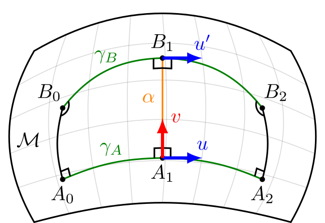
The positive-curvature proof constructs paired short geodesics using parallel transport, forming two Levi-Civita parallelogramoids. The retained curvature expansion makes each endpoint pair closer than the central pair for sufficiently small displacement, violating convexity of distance along the product geodesic.
The source’s final sentence calls this a “local minimum,” but the inequalities establish a larger midpoint than both endpoints. The summary follows those inequalities; the published equations and figure remain unchanged.
Equations
Appendix B Experiment Implementation Details
The implementation details clarify how manually selected regions, approximate optimization, and collision-checking choices affect the reported comparisons.
B.1 Planar Arm
The planar-arm graph contains nineteen regions. Start/goal and manually chosen narrow-passage seeds are supplemented with random collision-free seeds. The objective combines path length and duration.
The shown relaxed-and-rounded trajectories have lengths 7.749 and 8.448; branch-and-bound solutions have lengths 7.274 and 8.008. Thus the displayed plans are not the exact shortest results, although the exact second plan still needs more than a full turn of the middle joint.
B.2 KUKA iiwa Arm
The iiwa seeds cover reachable middle/top shelves and intermediate positions; bottom shelves are unreachable. Regions are prepared for empty and mug-holding hands and simplified by removing redundant inequalities. The objective combines time and path length, with continuous position, velocity, and acceleration plus hardware velocity limits. All shown trajectories use relaxation and rounding.
B.3 PR2 Bimanual Mobile Manipulator
The PR2 uses Drake’s robot description with convex hulls of link meshes for planning; reported collision annotations use the true mesh geometry. Shelf-target regions and manually selected intermediate regions are simplified, and irrelevant shelf-reaching regions are omitted for each query. GGCS again minimizes length plus duration using relaxation and rounding.
Drake-Trajopt uses B-splines and SNOPT. It first solves without collision constraints, then adds pointwise minimum-distance constraints at fifty trajectory samples, with a 1 mm target clearance and penalties beginning at 1 cm. Additional base-retreat waypoints are sometimes needed.
When initialized from a PRM trajectory, the optimizer uses one hundred collision samples and begins penalizing proximity at 1 m. These finite sampling choices explain why continuous-time collision avoidance differs from the region-based method even when an optimized curve looks shorter.