At a glance
SpaLoc scales hypergraph reasoning by combining sparse tensor representations, learned gates with a sparsity penalty, and local subgraph sampling. Information sufficiency estimates how much connecting-path information survives sampling and reduces positive training labels when that information is missing.
Experiments cover synthetic family relations and knowledge-graph link prediction. The method improves memory use and sampled-candidate prediction, but its success depends on local evidence and low relation arity. Its strong ranking scores use only fifty sampled negatives; performance deteriorates sharply when ranking against all entity replacements.
1 Introduction
Inferring a relation between two entities can require a third entity, as when a parent connects a grandparent and grandchild. Higher-order representations support such reasoning, but storing features for every triple costs cubic space in the number of entities.
SpaLoc exploits two assumptions: useful relations are sparse, and relevant evidence is usually nearby. It learns which intermediate hyperedges to retain, trains on sampled subgraphs, and adjusts labels for lost context. These mechanisms allow experiments on knowledge graphs with more than ten thousand nodes while operating on much smaller local subgraphs.
2 Related Work
Standard message-passing and embedding methods are efficient but have different representational limits from higher-order relational models. Inductive logic-programming systems can learn transferable relations, yet their search or tensor costs make large domains difficult.
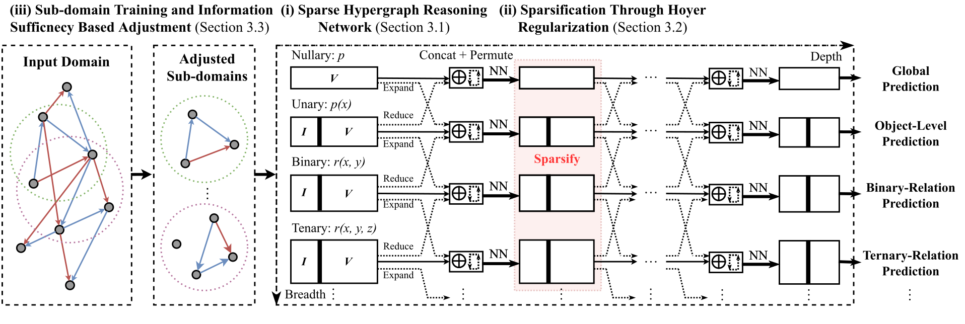
SpaLoc builds on sparse neural computation, Hoyer-style regularization, and graph sampling. Its regularizer acts on intermediate hyperedge gates rather than network weights. Its label adjustment addresses the fact that a sampled graph may remove evidence required for a positive full-graph relation. Figure 1 preserves the complete training pipeline.
3 SpaLoc Hypergraph Neural Networks
A hyperedge is an ordered tuple of entities, with an associated scalar or vector feature. Arity-one features describe nodes; arity-zero features describe the whole graph. Given input features such as parent relations, the network predicts a target feature either for all candidate edges or for one queried edge.
3.1 Sparse Hypergraph Neural Networks
The main backbone is a Neural Logic Machine (NLM), with an additional experiment on 2-GNNs. Each arity uses a coordinate-list sparse tensor: an index matrix records stored tuples, and a value matrix records their feature vectors. Unstored tuples represent zero vectors.
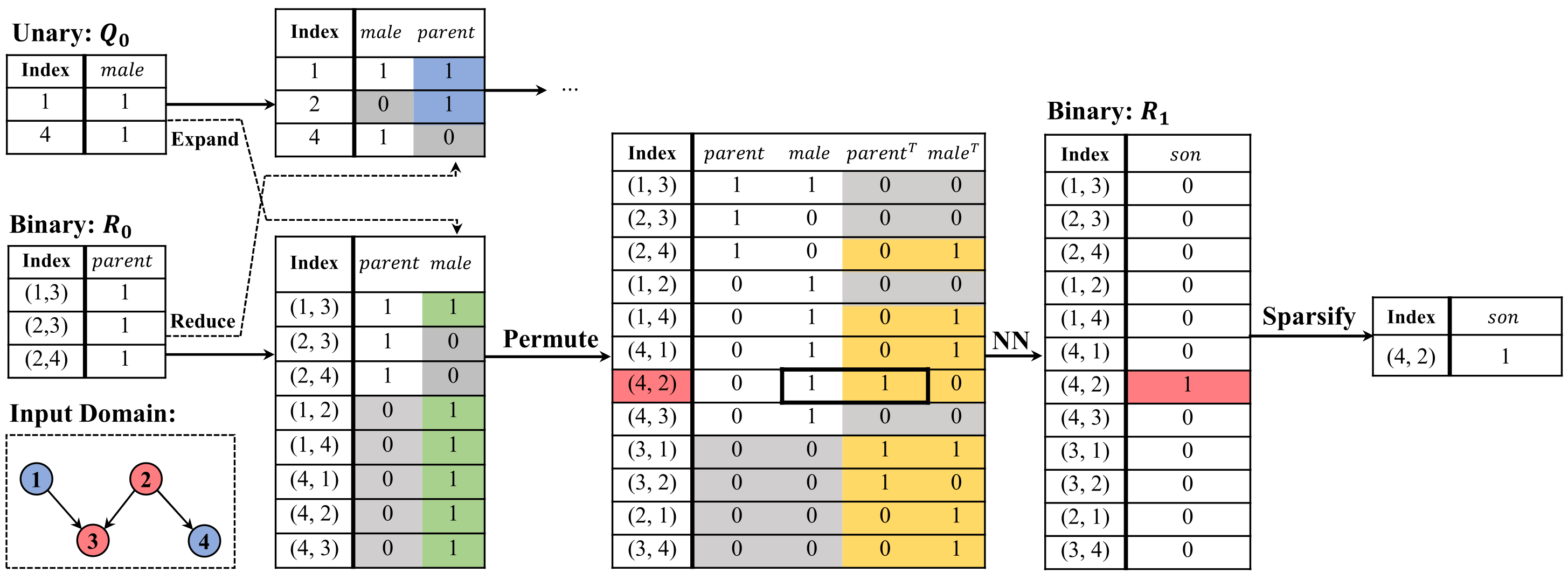
Each relational reasoning layer combines features at the same arity with expanded lower-arity and reduced higher-arity features. Expansion duplicates an entry across possible additional entities; reduction takes a maximum over the final entity. Concatenation aligns indices with zero padding, and permutation gathers every ordering of the same entities. The retained formulas and Figure 2 specify these operations. Permutation expands feature width by a factorial factor in arity.
A learned linear layer transforms the combined features. A separate sigmoid gate supplies one importance value per hyperedge, shared across its channels. Training multiplies the features by that gate; inference removes edges whose gate is below 0.05.
The useful sparsity pattern is not known before computation. Sparse storage alone therefore does not avoid all dense candidate expansion; the sparsity penalty and local sampling are essential. Higher-arity intermediates also remain useful when the input and output relations are only binary.
Equations
3.2 Sparsification through Hoyer Regularization
The paper defines a normalized Hoyer density measure and uses its squared norm-ratio form for training. Hoyer-Square ranges from one for a single nonzero entry to the vector length for equal-magnitude entries, favoring concentration into fewer active gates. It is scale-invariant, so the ratio alone does not fix the absolute size of surviving gate values.
The density loss sums Hoyer-Square scores across gate tensors and divides by their total size. Training adds it to the task loss with coefficient 0.01. The original measures and objective are retained, and Appendix D compares them with L1 and L2 penalties.
Equations
3.3 Subgraph Training
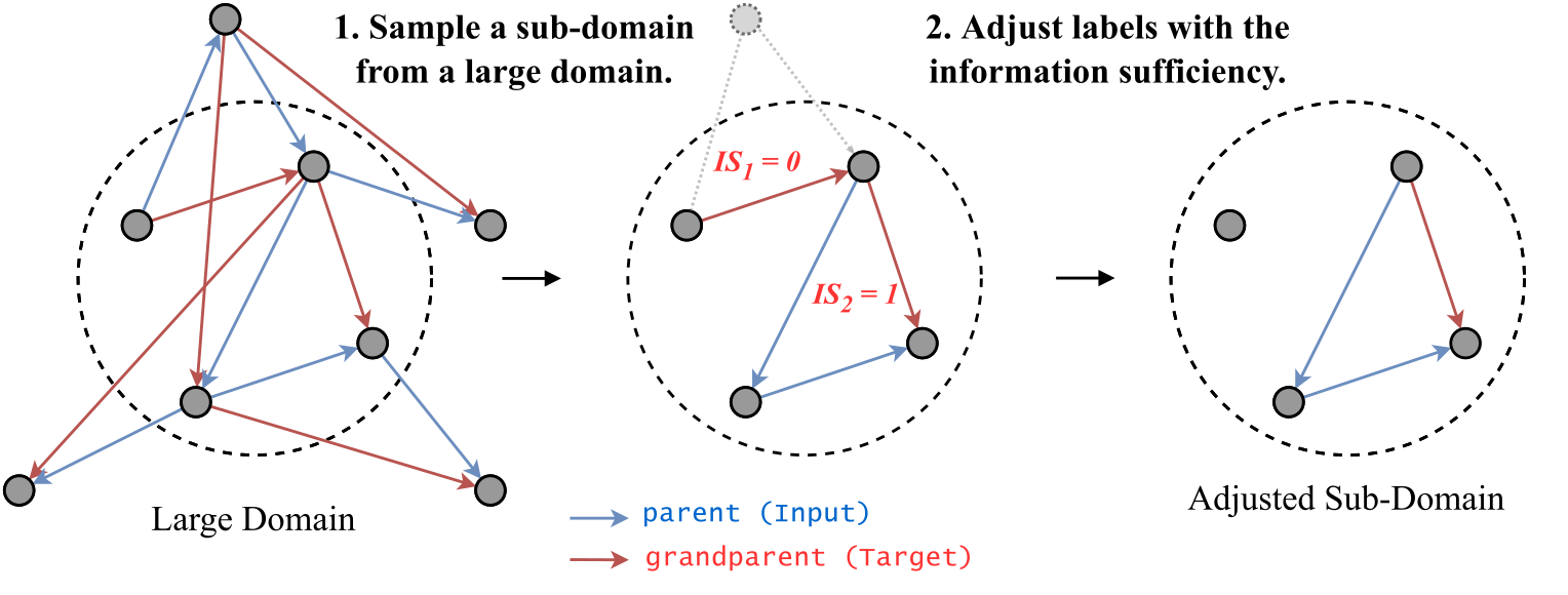
Sampling reduces training cost by retaining a local induced subgraph. Figure 3 illustrates the resulting problem: a positive relation in the full graph may become unsupported after its connecting evidence is removed. SpaLoc measures retained connectivity and adjusts the training target accordingly.
Information sufficiency
A hyperpath is a sequence of overlapping hyperedges whose union contains the queried entities. Information sufficiency (IS) is the ratio of connecting paths in the sampled subgraph to those in the full graph, with 0/0 defined as one.
In practice, counts are restricted by a task-dependent path-length threshold. Full-graph counts can be cached; sampled counts are recomputed locally. Adjacency or incidence-matrix powers provide the calculation. This is a structural proxy for retained evidence, rather than a proof that every logical fact needed for the query remains available.
Equations
Subgraph sampling
Training uses neighbor expansion: choose seed nodes, repeatedly sample neighbors, then include all original hyperedges entirely contained in the selected node set. This tends to retain short connecting paths.
For a single queried pair at inference time, a path sampler instead selects connecting paths and induces a subgraph from their nodes. Thus large-domain evaluation does not require dense reasoning over every entity tuple in the original graph.
Training label adjustment with IS
For a binary target, multiply the original label restricted to the subgraph by its IS score and train against this soft target. Negative labels remain zero; positive labels are reduced when connecting evidence is missing. The main text describes binary cross-entropy, whereas the implementation appendix calls the loss Softmax-Cross-Entropy. The edition retains this terminology difference rather than assuming a fully specified loss implementation.
Equation
4 Experiments
Synthetic family trees isolate relational expressiveness, sparsity, and sampling choices. Knowledge-graph experiments then test inductive and transductive link prediction under a sampled-negative evaluation protocol.
4.1 Family Tree Reasoning
Inputs are Father, Mother, Son, and Daughter relations; Appendix H retains all seven target definitions. Table 1 compares training on twenty versus two thousand entities and testing on one hundred. SpaLoc reaches 100% per-class accuracy on most tasks and 98.01% on HasSister after large-domain training. NLM and differentiable ILP match many small-domain results but cannot run the larger training setting on the specified 24 GB GPU.
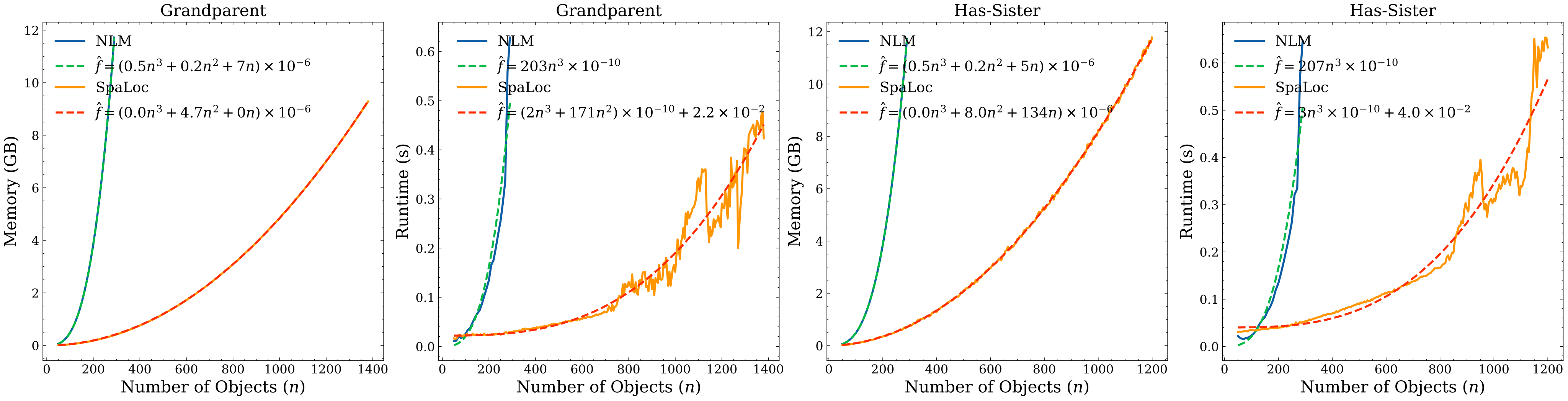
Figure 4 reports empirical time and memory curves for HasSister and Grandparent. The fitted curves suggest approximately quadratic rather than cubic memory growth; this is an observed scaling result, not a proven bound.
Table 2 shows benefits for both backbones at two hundred test entities. On Grandparent, SpaLoc+NLM reduces reported inference time from 135.0 to 23.9 ms and memory from 3,846 to 181 MB while retaining perfect accuracy.
Table 3 compares twenty-node training samples from increasingly large graphs. Uniform node sampling eventually loses almost all useful connecting evidence; random-walk and neighbor sampling retain high information sufficiency and perfect Grandparent accuracy. Neighbor expansion is not uniformly superior to random walks on every reported sufficiency score.
| Family Tree | MemNN | ILP | NLM | GraIL (R-GCN) | SpaLoc (Ours) | |||||
| 20 | 2,000 | 20 | 2,000 | 20 | 2,000 | 20 | 2,000 | 20 | 2,000 | |
| HasFather | 65.24 | - | 100 | - | 100 | - | 100 | 100 | 100±0.00 | 100±0.00 |
| HasSister | 66.21 | - | 100 | - | 100 | - | 97.05 | 97.95 | 100±0.00 | 98.01±0.04 |
| Grandparent | 64.57 | - | 100 | - | 100 | - | 99.95 | 98.08 | 100±0.00 | 100±0.00 |
| Uncle | 64.82 | - | 100 | - | 100 | - | 97.87 | 96.50 | 100±0.00 | 100±0.00 |
| MGUncle | 80.93 | - | 100 | - | 100 | - | 54.67 | 71.29 | 100±0.00 | 100±0.00 |
| FamilyOfThree | - | - | - | - | 100 | - | - | - | 100±0.00 | 100±0.00 |
| ThreeGenerations | - | - | - | - | 100 | - | - | - | 100±0.00 | 100±0.00 |
| Uncle | Grandparent | |||||
| Acc. | Time | Mem. | Acc. | Time | Mem. | |
| NLM | 100 | 133.8 | 3,846 | 100 | 135.0 | 3,846 |
| SpaLoc + NLM | 100 | 37.2 | 214 | 100 | 23.9 | 181 |
| 2-GNN | 100 | 145.1 | 5,126 | 100 | 145.5 | 5,126 |
| SpaLoc + 2-GNN | 100 | 23.7 | 645 | 100 | 19.2 | 519 |
| Node | Walk | Neighbor | ||||
| Acc | MIS | Acc | MIS | Acc | MIS | |
| 20 / 50 | 100 | 54.82 | 100 | 85.14 | 100 | 89.78 |
| 20 / 200 | 100 | 33.05 | 100 | 71.51 | 100 | 80.60 |
| 20 / 500 | 58.18 | 27.27 | 100 | 78.22 | 100 | 78.70 |
| 20 / 1,000 | 1.84 | 24.49 | 100 | 77.18 | 100 | 78.38 |
| 20 / 2,000 | 0 | 19.66 | 100 | 79.69 | 100 | 78.53 |
4.2 Real-World Knowledge Graph Reasoning
Inductive tests use disjoint training and evaluation subgraphs from WN18RR, FB15k-237, and NELL-995, each with four size variants. Table 4 reports higher AUC-PR for SpaLoc than the listed comparisons on all twelve variants. Appendix B gives standard errors over three seeds.
Transductive evaluation uses the standard graph splits, with NELL-995 following GraIL. SpaLoc still uses an inductive architecture without storing a learned embedding for each entity. Table 5 shows strong AUC-PR on all three datasets and strong Hits@10 on WN18RR and NELL-995. On FB15K-237, its 96.96% Hits@10 is below the roughly 98.7–98.9% embedding-model results.
Hits@10 ranks a true triplet against fifty randomly sampled negatives. The authors explicitly report near-zero ranking scores when the negative candidate set expands to all head/tail replacements. The small-candidate results therefore do not establish competitive performance under full-entity knowledge-graph ranking.
| Model | WN18RR | FB15k-237 | NELL-995 | |||||||||
| v1 | v2 | v3 | v4 | v1 | v2 | v3 | v4 | v1 | v2 | v3 | v4 | |
| Neural-LP | 86.02 | 83.78 | 62.90 | 82.06 | 69.64 | 76.55 | 73.95 | 75.74 | 64.66 | 83.61 | 87.58 | 85.69 |
| DRUM | 86.02 | 84.05 | 63.20 | 82.06 | 69.71 | 76.44 | 74.03 | 76.20 | 59.86 | 83.99 | 87.71 | 85.94 |
| RuleN | 90.26 | 89.01 | 76.46 | 85.75 | 75.24 | 88.70 | 91.24 | 91.79 | 84.99 | 88.40 | 87.20 | 80.52 |
| GraIL | 94.32 | 94.18 | 85.80 | 92.72 | 84.69 | 90.57 | 91.68 | 94.46 | 86.05 | 92.62 | 93.34 | 87.50 |
| TACT | 96.15 | 97.95 | 90.58 | 96.15 | 88.73 | 94.20 | 97.10 | 98.30 | 94.87 | 96.58 | 95.70 | 96.12 |
| SpaLoc | 98.45 | 99.96 | 96.63 | 99.34 | 99.74 | 99.34 | 99.55 | 99.29 | 100 | 98.56 | 97.19 | 97.34 |
| WN18RR | NELL-995 | FB15K-237 | ||||
| AUC-PR | H@10 | AUC-PR | H@10 | AUC-PR | H@10 | |
| TransE | 93.73 | 88.74 | 98.73 | 98.50 | 98.54 | 98.87 |
| DistMult | 93.08 | 85.35 | 97.73 | 95.68 | 97.63 | 98.67 |
| ComplEx | 92.45 | 83.98 | 97.66 | 95.43 | 97.99 | 98.88 |
| RotatE | 93.55 | 88.85 | 98.54 | 98.09 | 98.53 | 98.81 |
| GraIL | 90.91 | 73.12 | 97.79 | 94.54 | 92.06 | 75.87 |
| SpaLoc | 96.74 | 99.94 | 99.25 | 98.93 | 99.69 | 96.96 |
5 Conclusion
Sparse gates and local subgraphs make higher-order relational models practical for the evaluated tasks. The limitations follow directly from those assumptions: distant evidence or long chains can be missed, permutation cost grows factorially with arity, and the learned complexity lacks a general theoretical guarantee. The method is unsuitable without modification for extremely high-arity relations such as arity-67 WD50K examples.
Support came from ONR, NSF, AFOSR, MIT research programs, Stanford HAI, and industry sponsors; the authors distinguish their conclusions from sponsor views.
Appendix A Experimental configuration
Table 6 preserves every depth, breadth, hidden dimension, batch size, sample size, and path threshold. Experiments use Adam with learning rate 0.005, maximum arity three, linear transformations without hidden layers, and sigmoid activations. Family-tree models have five layers and twenty-node subgraphs; knowledge-graph models have six layers and ten- or twenty-node subgraphs.
The gate threshold is 0.05, selected using validation accuracy; the authors report similar behavior between 0.01 and 0.1. The sparsity-loss coefficient is 0.01 throughout. Arity three permits intermediate reasoning over triples, but the finite-depth model and locality assumptions still constrain which computations it can perform.
| Tasks | Depth | Breadth | Hidden Dims | Batch size | Subgraph size | ||
| Family Tree | HasFather | 5 | 3 | 8 | 8 | 20 | 1 |
| HasSister | 5 | 3 | 8 | 8 | 20 | 2 | |
| Grandparent | 5 | 3 | 8 | 8 | 20 | 2 | |
| Uncle | 5 | 3 | 8 | 8 | 20 | 2 | |
| MGUncle | 5 | 3 | 8 | 8 | 20 | 2 | |
| Family-of-three | 5 | 3 | 8 | 8 | 20 | 2 | |
| Three-generations | 5 | 3 | 8 | 8 | 20 | 2 | |
| Inductive KG | WN18RR | 6 | 3 | 64 | 128 | 10 | 3 |
| FB15K-237 | 6 | 3 | 64 | 64 | 20 | 3 | |
| NELL-995 | 6 | 3 | 64 | 128 | 10 | 3 | |
| Transductive KG | WN18RR | 6 | 3 | 64 | 64 | 20 | 3 |
| FB15K-237 | 6 | 3 | 64 | 64 | 20 | 3 | |
| NELL-995 | 6 | 3 | 64 | 64 | 20 | 3 |
Appendix B SpaLoc’s results with standard errors
Tables 7 and 8 retain all three-seed means and standard errors for inductive and transductive results. Small standard errors indicate consistency across these seeds under the reported protocol; they do not address the separate full-ranking failure.
Appendix C Implementation of subgraph samplers
For sampling only, a hypergraph is projected to a binary graph by connecting nodes that share a hyperedge. Neighbor expansion or path search selects nodes in this projection. The induced training graph then restores the original hyperedges whose complete node sets were selected, preserving their arities.
Appendix D Ablation study on sparsification loss
Table 9 compares L1, L2, and Hoyer-Square regularization on one-hundred-object test domains. Hoyer-Square reaches 100% accuracy on HasSister, Grandparent, and Uncle with intermediate densities of 0.51%, 0.48%, and 0.87%. It balances accuracy and sparsity better in these experiments, although L1 produces a slightly sparser HasSister representation with lower accuracy.
| HasSister | Grandparent | Uncle | ||||
| Accuracy | Density | Accuracy | Density | Accurcay | Density | |
| 91.81 | 0.48% | 99.8% | 0.99% | 74.69% | 0.68% | |
| 100 | 0.75% | 100% | 0.61% | 94.46% | 2.44% | |
| 100 | 0.51% | 100% | 0.48% | 100% | 0.87% | |
Appendix E Ablation study on SpaLoc’s maximum arity
Tables 10 and 11 compare maximum arity two versus three. Ternary intermediates substantially improve family-tree accuracy and the sampled knowledge-graph AUC-PR, including an Uncle increase from 50 to 100%. The result supports higher-order intermediate features even for binary input/output relations; it does not establish scalability to arbitrarily high arity.
| HasSister | Grandparent | Uncle | |
| Max Arity = 2 | 87.66 | 86.74 | 50.00 |
| Max Arity = 3 | 100 | 100 | 100 |
Appendix F Ablation Study on Label Adjustment
Table 12 compares no calibration, a constant 0.9 multiplier on positive labels, and IS-based adjustment for each sampler. IS with neighbor sampling gives 100% HasFather and 98.01% HasSister accuracy. The benefit is not universal: uniform node sampling remains at 50% on HasFather even with IS, showing that label adjustment cannot always recover from missing context.
Appendix G Calculation of the information sufficiency
The appendix uses a node–hyperedge incidence matrix and its matrix-power construction to count connecting traversals. The original k-hop incidence and unary/binary counting formulas are retained below. Such matrix powers count walks with multiplicity, including repeated vertices; the paper calls them hyperpaths and uses their ratio as the operational sufficiency score.
Equations
Appendix H Definition of Relations in Family Tree
The benchmark simulates family growth, assigning each new member a gender and either a pair of parents or no parents. Labels are computed from the published logical definitions retained below. The formulas preserve the source’s argument ordering and its capitalization of Parent/parent, rather than replacing them with informal kinship interpretations.