Overview
This extended abstract studies how tuple arity, depth, precision, and aggregation affect relational neural networks. Appendix A formalizes the architectures and their reductions; Appendix B supplies hierarchy arguments and graph-problem examples; Appendix C tests size generalization on synthetic graphs.
At a glance
The paper relates higher-order graph networks and Neural Logic Machines, characterizes a strict arity hierarchy through logic and Weisfeiler–Leman tests, and gives an example where higher arity reduces required depth. Its general depth hierarchy remains a conjecture. A separate finite-hypothesis argument shows eventual exact size generalization under exhaustive small-graph training, realizability, fixed precision, and perfect fitting. Synthetic experiments illustrate the distinction between expressibility, successful optimization, and extrapolation to larger graphs.
1 Introduction
Low-arity inputs do not imply that low-arity internal representations suffice. Tuple features can express relationships that node or pair features cannot distinguish. The work asks which arity and depth a task needs, then separately asks when learning on small graphs transfers to larger ones. Its structural-generalization result is conditional on a strong enumerative training setting; ordinary sampled gradient training is studied empirically rather than covered by an unconditional extrapolation guarantee.
2 Hypergraph Reasoning Problems and Hypergraph Neural Networks
A graph representation assigns features to every tuple of up to a chosen arity, including an arity-zero global feature. Outputs can be graph labels, node labels, or relation features. The studied higher-order graph network replaces one position of a tuple with every possible node and aggregates those neighbors. Neural Logic Machines instead combine expansion, reduction, permutation, and shared neural transformations across arities.
The stated equivalence maps a B-ary higher-order graph network to a maximum-(B+1)-arity NLM. This convention matters: the two models’ arity labels differ by one. The framework allows constant arity with graph-size-dependent depth and distinguishes bounded from unbounded precision. Expressiveness concerns existence of parameters, not whether an optimizer discovers them.
3 Expressiveness of Relational Neural Networks
Arity. For each maximum arity B, sufficiently deep (B+1)-ary NLMs strictly contain the B-ary family. The argument applies separately within fixed- and unbounded-precision settings; it does not order every model across those precision regimes. With suitable aggregation, counting first-order formulas using at most B variables can be realized at arity B, while some require more than B−1. The counting construction uses sum aggregation, so it should not be conflated with arbitrary-size exact counting in a fixed finite output range.
Depth. A proposed strict hierarchy for fixed precision and depth growth rates separated by a logarithmic factor is explicitly Conjecture 3.3. The cited congested-clique result has different precision/communication assumptions and does not prove it. For unbounded precision, the paper argues expressiveness saturates by O(nB−1) depth at arity B.
Concrete tradeoff. Bounded-distance source-to-target connectivity requires depth growing linearly with path bound k at arity two, whereas arity three can use repeated composition in O(log k) depth. This task-specific separation is stronger evidence than the unproved general hierarchy. The source’s phrase “at least O(k)” is a lower-bound statement; its no-o(k) formulation is the intended claim.
4 Learning and Generalization in Relational Neural Networks
Fixed-precision aggregation has a finite output range independent of set size; max and rounded mean qualify, while exact unbounded sum does not. Complete presentation supplies every labeled graph up to some size, including every assignment from a finite feature domain. This is much stronger than a finite random training sample.
Theorem 4.1 assumes the target is representable by the fixed-precision model family and that training achieves zero error on a sufficiently large complete presentation. The proof relies on a fixed finite set of distinct hypotheses: each wrong hypothesis has a finite counterexample, and the largest required counterexample size gives a sufficient cutoff. The result establishes existence of such a cutoff, not an efficient sample bound, practical exhaustive enumeration, or a guarantee that gradient descent fits the data. It does not prove arbitrary continuous/noisy-domain generalization.
Equation
5 Related Work
The analysis connects relational architectures to circuits, distributed computation, graph-isomorphism refinement, and bounded-variable logic. WL-based graph-network expressiveness and logical characterizations support the arity discussion. Algorithmic-alignment work studies extrapolation and sample complexity on particular algorithms; this paper’s complete-presentation result instead uses finite precision and a finite hypothesis family. These are complementary conclusions with different assumptions.
6 Conclusion
Higher-order tuple representations can increase expressiveness and reduce depth needed for particular graph tasks, at greater computation cost. Exact structural generalization is established only under the finite-domain, fixed-family, exhaustive-training assumptions, while practical experiments show both successes and failures. The general fixed-precision depth hierarchy, continuous/noisy inputs, and reliable optimization remain unresolved. The authors acknowledge ONR, NSF, AFOSR, CBMM, and MIT research support.
Appendix A Hypergraph Neural Networks
Two architecture descriptions and explicit simulation reductions establish the paper’s expressiveness convention. The section also distinguishes all-tuple networks from cheaper node–hyperedge message passing and states the cost of retaining higher-order features.
A.1 Higher-order Graph Neural Networks
A B-ary higher-order graph network stores a feature for every B-tuple. For each candidate node, it collects tuples obtained by replacing each coordinate, concatenates their features with the current tuple, transforms them, and aggregates messages. This all-tuple construction is richer and more expensive than updating only listed hyperedges. The original neighborhood and aggregation equations are preserved, including the source’s indexing notation.
Equations A.1–A.4
| (A.1) |
| (A.2) | |||||
| (A.3) |
| (A.4) |
A.2 Neural Logic Machines
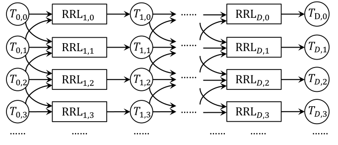
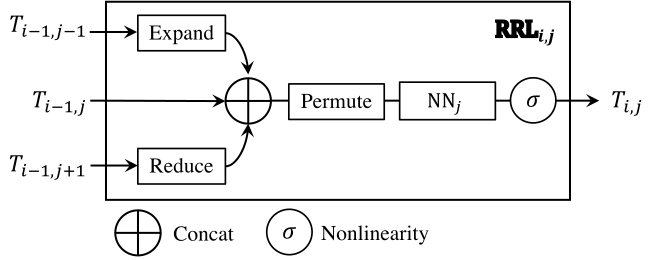
An NLM stores tensors for arities zero through B. Each block expands features from the next lower arity, reduces over a variable from the next higher arity, concatenates these with same-arity features, gathers argument permutations, and applies a neural transformation. Reduction outputs arity j; the source prose’s j+1 output statement is inconsistent with its own displayed indexing. Sharing transformations across layers permits recurrence, although simulating distinct layers may require increased width. Full architecture panels and mathematical operations remain below.
Equations
A.3 Expressiveness Equivalence of Relational Neural Networks
Lemma A.1 simulates D distinct width-W layers by D repetitions of one wider transformation, using (D+1)(W+1) state dimensions and activation flags to route layer-specific computation. Thus weight sharing can preserve a fixed-depth computation with additional storage. Since width grows with D in this construction, it is not a free constant-width reduction for arbitrarily increasing depth. Expressiveness reductions require identical outputs on every input and apply to regression as well as classification.
Equivalence between HO-GNNs and NLMs.
A B-ary higher-order graph layer is simulated by two NLM layers at arity B+1: expand and permute to collect each replacement tuple, compute its message, then reduce the added variable. This gives depth 2D for a depth-D source network.
The reverse reduction stores lower-arity tuple permutations inside B-tuple features and uses broadcast messages to simulate reduction. Its highest-arity argument assumes those features arise from lower-arity expansion, and can retain previous-layer representations in wider features. The stated result uses at most D higher-order graph iterations. These constructions establish the paper’s architecture equivalence with the one-arity offset; they do not assert equal parameter counts, constant storage overhead for all growing depths, or equal learnability under gradient training.
Equations A.5
| (A.5) |
A.4 Expressiveness of hypergraph convolution and attention
Node–hyperedge convolution and attention first aggregate node features into each incident edge, then return edge messages to nodes. The paper shows how all-tuple NLM operations can simulate these steps. The reverse need not hold: identical node features in two disjoint triangles cannot tell a within-triangle triple from a mixed triple, while ternary tuple features can. Its stated O(|V||E|) message-passing cost contrasts with O(|V|B) all-tuple computation; precise sparse implementations can depend on incidence structure.
Equations A.6–A.7
| (A.6) |
| (A.7) |
A.5 The Time and Space Complexity of NLMs
With feature width and arity treated as constants, each all-tuple layer costs O(nB), giving O(DnB) time. Retaining the entire history for backpropagation has the same space order; that statement is not a necessary inference-memory bound. The equivalent higher-order graph network stores one fewer tuple dimension but broadcasts over n replacement nodes, giving the same stated time order.
Appendix B Arity and Depth Hierarchy: Proofs and Analysis
The appendix separates proved arity and connectivity statements from conjectured lower bounds. Its catalog provides useful constructions, but not every “minimum” entry has a matching proof.
B.1 Proof of Theorem 3.1 : Arity Hierarchy.
The reduction to higher-dimensional Weisfeiler–Leman separation examples supplies graph pairs indistinguishable at arity B but distinguishable at B+1. Higher arity can also ignore its extra features and emulate lower arity. Together these give strict containment once sufficient depth is available. The conclusion concerns the studied all-tuple architectures and their specified aggregation power.
B.2 Upper Depth Bound for Unbounded-Precision NLM.
For a fixed graph size, the higher-dimensional WL test partitions inputs into indistinguishability classes and stabilizes within a polynomial number of rounds. Counting-logic formulas characterize those classes; an unbounded-precision NLM can evaluate them and assign outputs. The resulting bound is O(nB) for arity B+1, equivalent to the main text’s O(nB−1) at arity B. This unlimited-precision argument does not resolve the fixed-precision depth conjecture or provide a practical width bound.
B.3 Graph Problems
Counting and local structure. Sum aggregation counts colors; degree computation followed by pooling detects a three-node link or maximum degree. The paper’s “3-link” is a two-edge triple, despite a later length-three description. Its “4-link” permits a triangle because not all four positions must be distinct. Triangle detection is realizable by a four-layer ternary NLM; two triangles versus one six-cycle demonstrate a binary-arity limitation. Four-clique detection/counting has an arity-four construction, but the text does not prove the suggested impossibility at arity three.
Connectivity. Repeated propagation from a marked source gives linear-depth bounded-distance reachability at arity two. Ternary pair composition enables logarithmic depth through repeated squaring. The two-chain lower-bound proof shows that the marked endpoints cannot interact soon enough at lower arity. Theorem B.1’s statement omits its arity value and several displayed indices contain typographical inconsistencies; the notes use the explicit arity-two statement in the main text, leaving the original equations unchanged.
Other graph problems. Minimum aggregation and min-plus composition extend the constructions to distances. A Dinic-inspired discussion proposes a cubic-depth maximum-flow construction, while the table marks several lower bounds as conjectured. Treat this as a construction catalog with varying proof detail, not a complete set of tight optimal bounds.
| 4-Clique Detection NLM[, 4] | 4-Clique Count NLM[, 4] | |
| Triangle Detection NLM[,3] | All-Pair Distance NLM[, 3]⋆ | |
| Bipartiteness NLM[, 3]⋆ | ||
| All-Pair Connectivity NLM[, 3]⋆ | ||
| All-Pair Connectivity- NLM[, 3]⋆ | ||
| FOC2 Realization NLM[, 2] [14] | S-T Distance NLM[, 2] | |
| 3/4-Link Detection NLM[, 2] | Max Degree NLM[, 2] | |
| S-T Connectivity NLM[, 2] | Max Flow NLM[, 2]⋆ | |
| S-T Connectivity- NLM[, 2] | ||
| Node Color Majority: NLM[, 1] | Count Red Nodes: NLM[, 1] | |
| Classification Tasks | Regression Tasks |
Equations
Appendix C Experiments
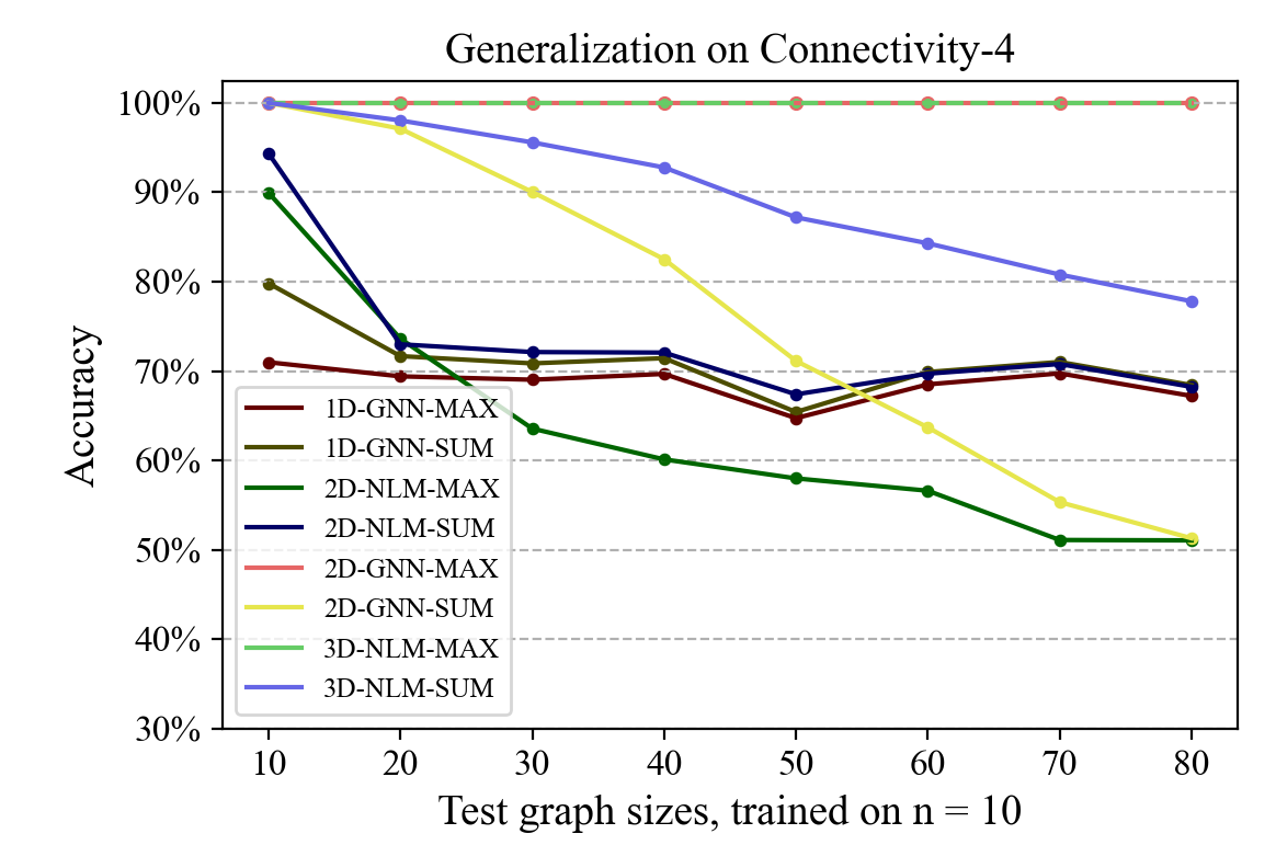
Synthetic experiments compare substructure classification, family-relation prediction, bounded connectivity, and unrestricted connectivity. They test gradient-trained models on larger sampled graphs, providing finite empirical evidence rather than implementing exhaustive complete presentation.
C.1 Experiment Setup
Each setting uses eight hundred training, one hundred validation, and three hundred test graphs per evaluated size. Random graphs vary edge density around n, 2n, n log n, and n²/2. Half the time, repeated components are constructed before adding random edges to create challenging symmetries. The resulting benchmark is deliberately structured rather than a uniform sample of all labeled graphs.
Substructure Detection.
Negative substructure examples add edges until a size limit or maximal forbidden-subgraph boundary is reached. Positive examples replace edges until the target substructure appears, keeping other graph properties similar. This reduces easy density cues relative to independently sampling positive and negative graphs.
Family Tree.
Family trees add people sequentially, either introducing an unrelated person or assigning a new child to an available woman–man pair. The parent-assignment probability varies with the current single-person fraction. These synthetic generation conventions define the grandparent/uncle test distribution; they are not a general demographic model.
Connectivity.
Connectivity uses similarly generated graphs with balanced positive and negative query pairs. Balancing the queried labels matters when interpreting the reported accuracies and their comparison across graph sizes.
C.2 Model Implementation Details
Most models use width 128; the largest tuple models use 64. Ordinary tasks use four distinct layers, while unrestricted connectivity repeats an internal layer a number of times sampled between two and three times log n. Training uses Adam for one hundred epochs at initial learning rate 3×10⁻⁴, decayed at epochs fifty and eighty. The setup says ReLU worked best across alternatives, while the results section states all reported models use sigmoid; that reporting inconsistency is retained rather than resolved by assumption.
C.3 Results
The tables report three-seed standard errors. Substructure models train on ten-node graphs and test at thirty nodes; family relations train at twenty and test at eighty; connectivity trains at ten and tests at eighty. These task-specific captions supersede the prose’s blanket ten-to-thirty description. Ternary max-pooling NLMs generalize perfectly on the reported link/triangle, family, and bounded-connectivity tests. Sum variants often fit small graphs yet deteriorate with size.
Expressibility is not sufficient for optimization: arity-four NLMs do not reliably learn perfect four-clique detection, reaching 82.0% at size ten and 93.1% at thirty with max aggregation. Equivalent architecture families also need not train equally well: the binary higher-order graph model stays near 71.9% on large unrestricted-connectivity tests, while the ternary max NLM reaches about 100%. Figure 2 shows bounded-connectivity accuracy through eighty nodes, not arbitrary-size verification. The finite synthetic successes support the proposed design choices without proving the exhaustive-training theorem applies to these sampled datasets.
| 3-link | 4-link | triangle | 4-clique | ||||||
| Model | Agg. | ||||||||
| 1-ary GNN | Max | 70.0±0.0 | 82.7±0.0 | 92.0±0.0 | 91.7±0.0 | 73.7±3.2 | 50.2±1.8 | 55.3±4.0 | 46.2±1.3 |
| Sum | 100.0±0.0 | 89.4±0.4 | 100.0±0.0 | 86.1±1.2 | 77.7±8.5 | 48.6±1.6 | 53.7±0.6 | 55.2±0.8 | |
| 2-ary NLM | Max | 65.3±0.6 | 54.0±0.6 | 93.0±0.0 | 95.7±0.0 | 51.0±1.7 | 49.2±0.4 | 55.0±0.0 | 45.7±0.0 |
| Sum | 100.0±0.0 | 88.3±0.0 | 100.0±0.0 | 67.4±16.4 | 82.0±2.6 | 48.3±0.0 | 53.0±0.0 | 54.4±1.5 | |
| 2-ary GNN | Max | 78.7±0.6 | 76.0±17.3 | 97.7±4.0 | 98.6±2.5 | 100.0±0.0 | 100.0±0.0 | 55.0±0.0 | 45.7±0.0 |
| Sum | 100.0±0.0 | 51.2±7.9 | 100.0±0.0 | 45.7±7.6 | 100.0±0.0 | 49.2±1.0 | 61.0±5.6 | 54.3±0.0 | |
| 3-ary NLM | Max | 100.0±0.0 | 100.0±0.0 | 100.0±0.0 | 100.0±0.0 | 100.0±0.0 | 100.0±0.0 | 59.0±6.9 | 45.9±0.4 |
| Sum | 100.0±0.0 | 87.6±11.0 | 100.0±0.0 | 65.4±14.3 | 100.0±0.0 | 80.6±8.8 | 73.7±13.8 | 53.3±8.8 | |
| 3-ary GNN | Max | 79.0±0.0 | 86.0±0.0 | 100.0±0.0 | 100.0±0.0 | 100.0±0.0 | 100.0±0.0 | 84.0±0.0 | 93.3±0.0 |
| Sum | 100.0±0.0 | 84.1±18.6 | 100.0±0.0 | 61.1±15.0 | 100.0±0.0 | 95.1±7.3 | 80.5±0.7 | 66.2±19.6 | |
| 4-ary NLM | Max | 100.0±0.0 | 100.0±0.0 | 100.0±0.0 | 100.0±0.0 | 100.0±0.0 | 100.0±0.0 | 82.0±1.7 | 93.1±0.2 |
| Sum | 100.0±0.0 | 59.1±5.3 | 100.0±0.0 | 67.7±24.1 | 100.0±0.0 | 82.1±12.8 | 84.0±0.0 | 67.0±18.9 | |
| grand parent | uncle | connectivity-4¶ | connectivity | ||||||
| Model | Agg. | ||||||||
| 1-ary GNN | Max | 84.0±0.3 | 64.8±0.0 | 93.6±0.3 | 66.1±0.0 | 72.6±3.6 | 67.5±0.5 | 85.6±0.3 | 75.1±1.9 |
| Sum | 84.7±0.1 | 64.4±0.0 | 94.3±0.2 | 66.2±0.0 | 79.6±0.1 | 68.3±0.1 | 87.1±0.3 | 75.0±0.2 | |
| 2-ary NLM | Max | 82.3±0.5 | 65.6±0.1 | 93.1±0.0 | 66.6±0.0 | 91.2±0.2 | 51.0±0.6 | 88.9±2.6 | 67.1±4.8 |
| Sum | 82.9±0.1 | 64.6±0.1 | 93.4±0.0 | 66.7±0.2 | 96.0±0.4 | 68.3±0.5 | 84.0±0.0 | 71.9±0.0 | |
| 2-ary GNN | Max | 100.0±0.0 | 100.0±0.0 | 100.0±0.0 | 100.0±0.0 | 100.0±0.0 | 100.0±0.0 | 84.0±0.0 | 71.9±0.0 |
| Sum | 100.0±0.0 | 35.7±0.0 | 100.0±0.0 | 33.9±0.0 | 100.0±0.0 | 51.3±5.3 | 84.0±0.0 | 71.9±0.0 | |
| 3-ary NLM | Max | 100.0±0.0 | 100.0±0.0 | 100.0±0.0 | 100.0±0.0 | 100.0±0.0 | 100.0±0.0 | 100.0±0.0 | 100.0±0.1 |
| Sum | 100.0±0.0 | 35.7±0.0 | 100.0±0.0 | 50.8±29.4 | 100.0±0.0 | 77.8±11.8 | 100.0±0.0 | 88.2±8.0 | |
| 3-ary NLM | Max | 100.0±0.0 | 100.0±0.0 | 100.0±0.0 | 100.0±0.0 | N/A | N/A | N/A | N/A |
| Sum | 100.0±0.0 | 35.7±0.0 | 100.0±0.0 | 33.8±29.4 | N/A | N/A | N/A | N/A | |