Overview
The complete paper and supplement are included, covering task semantics, planning and training algorithms, dependencies, datasets, baseline implementations, and computational costs.
At a glance
Rational Subgoals learns state classifiers for named goals from unsegmented demonstrations paired with structured instructions. A planning-based rationality objective jointly grounds the goal terms and aligns them to trajectory segments. Learned ordering dependencies suggest useful intermediate goals for longer tasks. Experiments in discrete crafting and continuous navigation environments show strong compositional planning results, under known transition models and deterministic, fully observed states.
Introduction
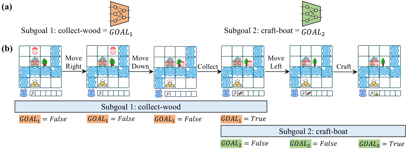
Long tasks become easier to search when useful intermediate achievements are available. RSGs represents each action term by a learned goal-state classifier rather than a fixed policy. Demonstration rationality helps identify when each goal was reached; empirical ordering patterns then suggest waypoints for new final goals. This separates reusable goal recognition from environment-model-based action search, allowing new instruction compositions while retaining substantial online planning cost.
Rational Subgoal Learning and Planning
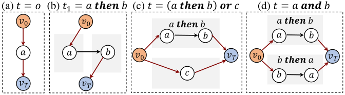
An atomic task requires a trajectory to start with its goal false and end with it true. The task language combines atoms with then, or, and and; then constrains completion order, or allows alternatives, and and allows different completion orders. A finite-state machine represents each instruction. Its states track current subgoals, while the environment state tracks the physical world. N-ary conjunction expands possible orders with subsets of completed goals, so automaton size can grow rapidly. The formal constructions and equations are retained.
Equations
Remark.
The implemented language describes finite tasks through a restricted temporal structure; it does not model infinite loops or unrestricted temporal specifications. Instructions are structured expressions rather than arbitrary natural-language sentences.
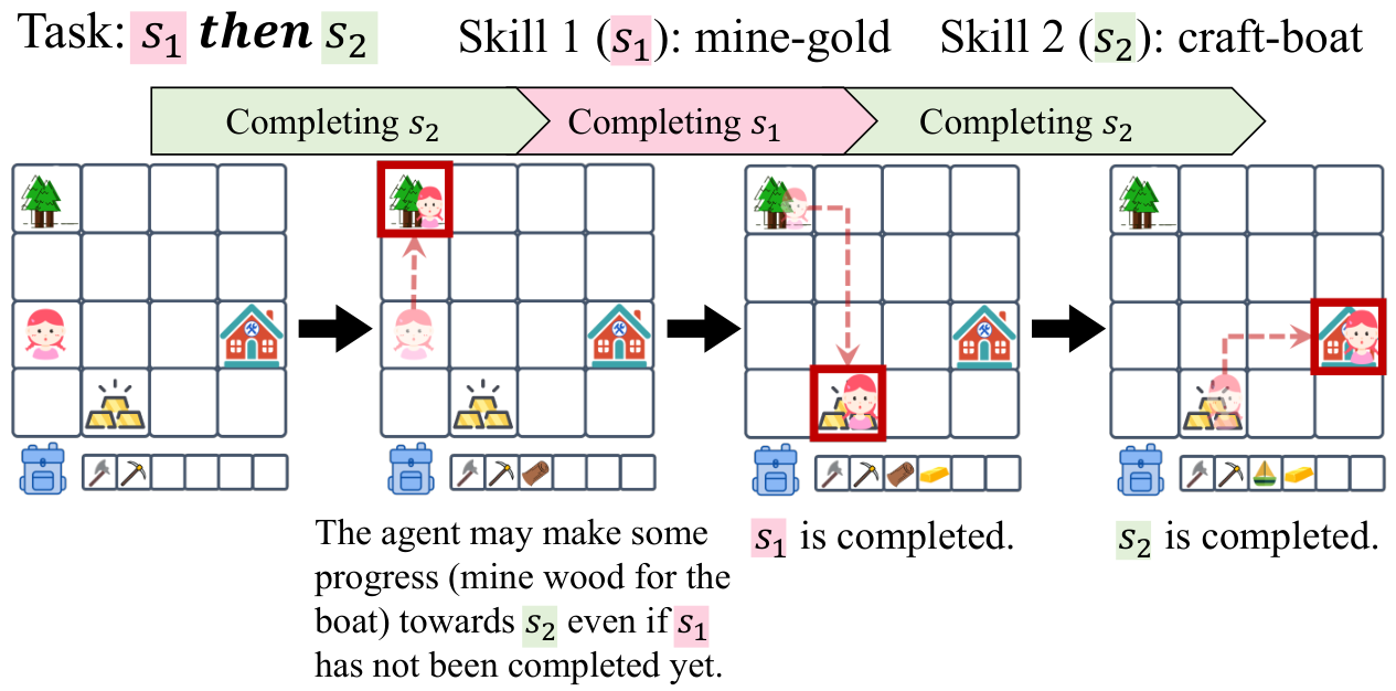
Execution steps for different subgoals can interleave.
Completion order does not prohibit preparatory actions for a later goal. An agent may collect wood for a boat, then mine gold, then finish the boat while satisfying mine-gold then craft-boat. This permits globally useful interleaving rather than concatenating independently optimal subgoal policies. Figure 3’s caption contains a repeated-label typo; the surrounding explanation and example specify the gold-before-boat order.
Planning with RSGs
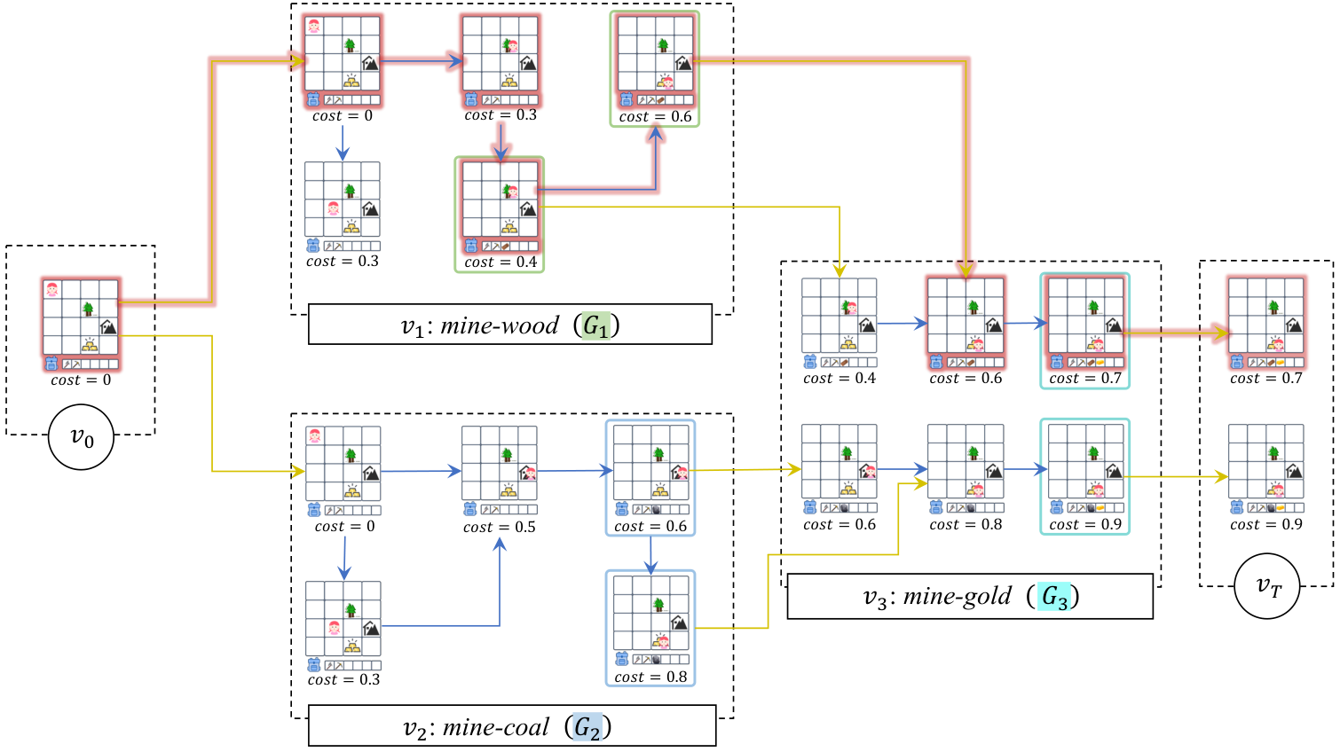
Planning searches a product of environment states and instruction-machine states. Environmental actions move the world; machine transitions mark subgoal completion. Costs combine physical action cost with penalties for inconsistent learned goal transitions. The formal transition requires the current goal true and the next goal not yet true; Figure 4’s caption incorrectly describes both as false. The implementation uses modified A* with effort distributed across subgoals, and sampling-based planning for continuous geometry. Its bounded/pruned search does not guarantee globally optimal plans, and learned soft classifiers do not guarantee true task completion outside their accuracy.
Equation
Example.
The worked search branches between mining wood and coal, then joins the gold-mining subgoal. Low-cost machine transitions occur where goal conditions permit them. The terminal trajectory is recovered by tracing back the lowest-cost reached terminal state.
Learning RSGs from Unsegmented Trajectories and Descriptions
For each candidate goal classifier, planning estimates cost-to-go and a soft-rational action likelihood. Dynamic programming finds the best latent assignment of observed states/actions to instruction-machine nodes. A contrastive term favors the paired instruction over randomly sampled alternatives. Gradients pass through the value and alignment computations to update goal classifiers. The method learns from high-level instruction labels without annotated subgoal boundaries, but assumes access to a world model and approximately rational demonstrations.
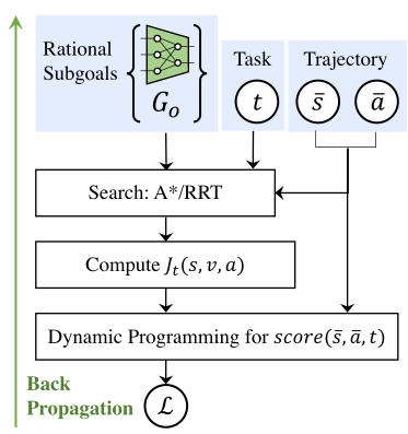
Equations 1–5
| (1) |
| (2) |
| (3) |
| (4) |
| (5) |
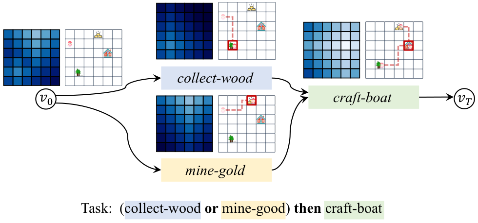
RSG Dependency Discovery and Planning
Dependency discovery counts which learned goals first become true before others in the training demonstrations, then normalizes these counts. These empirical ordering associations suggest useful predecessors; they are not verified causal preconditions. At test time, backward search proposes sequential instructions ending in the requested goal, prioritizing likely dependencies and shorter chains. The experiment caps chains at six subgoals, then invokes low-level planning for each candidate.
Equations 6–7
| (6) |
| (7) |
Experiments
Experiments compare goal-based learning with reward-based and policy-based alternatives in Crafting World (Chen, Gupta, and Marino, 2021) and Playroom (Konidaris, Kaelbling, and Lozano-Perez, 2018).
Crafting World.
Crafting World includes tool collection, resource mining, crafting, rivers, and doors. Training uses 26 primitive and 26 compositional tasks, with 400 demonstrations per task. Primitive-task demonstrations start with required tools already available. Evaluation separates new trajectories of seen compositions from 12 unseen compositions; the latter can have longer instructions.
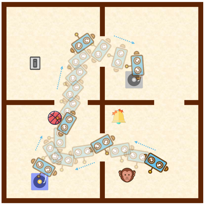
Playroom.
Playroom is a continuous two-dimensional configuration space with agent translation and rotation, obstacles, and six interactive objects. Interactions trigger automatically near objects. Six primitive and eight compositional training tasks are compared with eight novel tasks, again using 400 demonstrations per task. Obstacles have fixed geometry and locations in this experiment.
Baselines
Inverse reinforcement learning learns task-conditioned rewards; behavior cloning learns task-conditioned policies. BC-FSM adds the same instruction automata to policy learning. RSGs and the IRL baseline use the transition model, while the cloning baselines do not, so performance differences combine representation and access to model-based search.
Results
RSGs achieves 99.6% success on seen-composition Crafting World tasks and remains strong on novel compositions, where several baselines nearly fail. An image-state variant scores 82.0% and 78.2% on the two splits, compared with 38.2% and 31.5% for the reported BC-FSM comparison. The success rates are empirical under the stated search budgets; they do not imply universal task satisfaction or optimal plans.
| Model | Task Input | Env. Tran. | Crafting World | Playroom | ||
| Com. | Novel | Com. | Novel | |||
| IRL | Lang. | Y | 36.5 | 1.8 | 28.3 | 9.6 |
| BC | Lang. | N | 11.2 | 0.8 | 15.8 | 4.8 |
| BC-fsm | FSM | N | 5.2 | 0.3 | 38.2 | 31.5 |
| RSGs | FSM | Y | 99.6 | 97.8 | 82.0 | 78.2 |
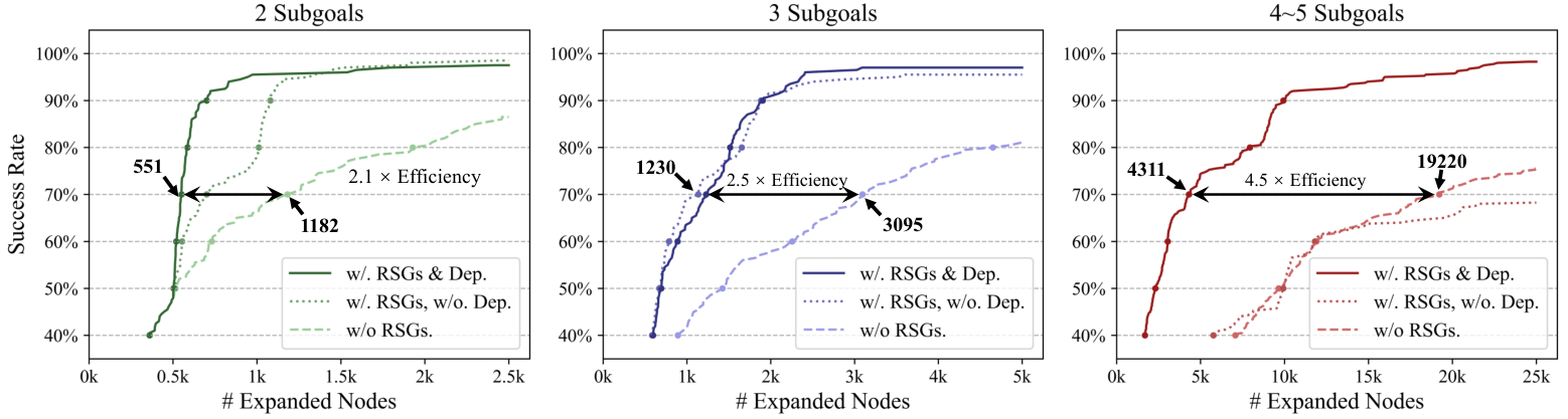
Planning with goals.
Final-goal evaluation uses eight manually selected goals requiring two to five intermediate subgoals, with 100 starting states each. Useful dependencies matter most for longer tasks: the reported 70%-success comparison needs 4,311 expanded nodes with the learned guidance versus 19,220 for blind search. Uniform subgoal guidance can perform worse than blind search by wasting effort on poor instruction candidates. The curves measure expanded search nodes, not an architecture-independent runtime speedup.
Related Work
Related work learns modular policies, options, reward functions, symbolic task structure, or unlabeled subgoals. RSGs instead grounds explicitly named goal conditions and replans their realization from the environment model. Its inverse-planning objective aligns demonstrations through rationality rather than action similarity alone. Combining labeled and unlabeled trajectories is left open.
Conclusion
Reusable goal classifiers and learned ordering associations support compositional planning in the evaluated domains. The framework’s strength is separating goal grounding from task-specific execution through planning.
Limitation.
The method assumes deterministic, fully observed dynamics and cannot currently learn from trajectories lacking task descriptions. Stochastic domains would need algorithmic changes, potentially including causal-entropy objectives and stochastic planning. Online search, imperfect learned goal tests, finite task-language scope, and combinatorial instruction generation remain practical limits. The authors acknowledge the listed collaborators and research sponsors.
Appendix A Implementation Details of RSGs
Re-parameterize 1 − G o ( ⋅ ) using a separate neural network.
Training uses a separate initial-condition network I rather than forcing it to equal 1−G. This relaxation stabilizes fitting and permits different equivalent goal/initial-condition representations. The reported planning success falls from 99.6% to about 75% when one complementary classifier is used. At execution time, the implementation uses the goal classifier and ignores the separate initial-condition network.
Equations
fsm - A ∗
A ∗ at each fsm node.
Within each machine node, search begins with breadth-first expansion—depth three in training and four in testing—then uses heuristic-guided search for 15 or 25 additional layers. It retains only the best ten candidates per node and layer. Task-specific value approximators learn from search-tree value iteration; unseen test tasks use a zero heuristic. These pruning choices trade exhaustive search for efficiency.
Search on an fsm .
The product search starts at the initial world/machine state, expands subgoal nodes in topological order, then attempts outgoing machine transitions. The appendix describes up to 5,000 A* steps per machine node and selects the lowest-cost reached terminal trajectory.
Optimality of the A* algorithm on fsm .
The appendix explicitly states that balancing expansion across machine nodes can return suboptimal plans even with a perfect heuristic. Standard optimality requires appropriate global best-first expansion with admissible bounds, or continuing until no unexpanded node can improve the solution. The tested implementation prioritizes computational efficiency.
Transitions on fsm
Alignment dynamic programming chooses the highest-scoring latent machine-transition sequence. With soft goal scores this differs from averaging over stochastic transitions; the two coincide only for binary goal conditions. The alternative expected-rationality formulation could use stochastic planning but may increase computation. Algorithm 3 retains the full implemented recurrence.
Discover and search with dependencies
Evaluate goal classifiers when computing first ( s ¯ , o ) for discovering dependencies.
Dependency discovery thresholds each soft goal classifier using its minimum and maximum outputs on training states. The source specifies the product MinG×MaxG as the threshold; that original rule is retained rather than replaced with a midpoint or a universal 0.5 cutoff.
Tuning hyperparameters.
Experiments use action cost 0.1, transition-cost weight 1, inverse rationality 1, contrastive weight 0.1, and classification temperature parameter 1. The appendix reports moderate robustness over the explored ranges, while noting sensitivity to transition cost relative to expected subgoal length.
Scalability and complexity of instruction generating.
The simplified complexity argument compares enumerating m subgoals and locally realizing each in l actions with searching all ml primitive steps directly. The proposed benefit assumes the subgoal vocabulary is much smaller than the number of local primitive sequences; candidate instruction enumeration still grows exponentially with m.
Appendix B Dataset
Crafting World
The modified crafting domain has 47 object types and 27 mining/crafting rules. Several recipes share a station. Keys or switches handle doors, and boats permit river crossing. Interaction depends on colocated objects, inventory capacity, and required tools.
| Primitive | |||
| grab-pickaxe | grab-axe | grab-key | toggle-switch |
| craft-wood-plank | craft-stick | craft-shears | craft-bed |
| craft-boat | craft-sword | craft-arrow | craft-cooked-potato |
| craft-iron-ingot | craft-gold-ingot | craft-bowl | craft-beetroot-soup |
| craft-paper | mine-gold-ore | mine-iron-ore | mine-sugar-cane |
| mine-coal | mine-wood | mine-feather | mine-wool |
| mine-potato | mine-beetroot | ||
| Compositional | |||
| grab-pickaxe | grab-axe | ||
| grab-key | toggle-switch | ||
| mine-wood then craft-wood-plank | craft-wood-plank then craft-stick | ||
| craft-iron-ingot or craft-gold-ingot then craft-shears | mine-wool and craft-wood-plank then craft-bed | ||
| craft-wood-plank then craft-boat | craft-iron-ingot and craft-stick then craft-sword | ||
| mine-feather and craft-stick then craft-arrow | mine-potato and mine-coal then craft-cooked-potato | ||
| mine-iron-ore and mine-coal then craft-iron-ingot | mine-gold-ore and mine-coal then craft-gold-ingot | ||
| craft-wood-plank or craft-iron-ingot then craft-bowl | craft-bowl and mine-beetroot then craft-beetroot-soup | ||
| mine-sugar-cane then craft-paper | grab-pickaxe then mine-gold-ore | ||
| grab-pickaxe then mine-iron-ore | grab-pickaxe or grab-axe then mine-sugar-cane | ||
| grab-pickaxe then mine-coal | grab-axe then mine-wood | ||
| craft-sword then mine-feather | craft-shears or craft-sword then mine-wool | ||
| grab-axe or mine-coal then mine-potato | grab-axe or grab-pickaxe then mine-beetroot | ||
| Novel | |||
| 1. mine-sugar-cane then craft-paper | |||
| 2. mine-potato and (gran pickaxe then mine-coal) and craft-cooked-potato | |||
| 3. mine-beetroot and (grab-axe then mine-wood then craft-wood-plank then craft-bowl) then craft-beetroot-soup | |||
| 4. grab-axe then mine-wood then craft-wood-plank then grab-pickaxe then mine-iron-ore and mine-coal then craft-iron-ingot then craft-shears then mine-wool then craft-bed | |||
| 5. grab-axe then mine-wood then craft-wood-plank then craft-stick then grab-pickaxe then mine-iron-ore and mine-coal then craft-iron-ingot then craft-sword then mine-feather then mine-wood then craft-wood-plank then craft-stick then craft-arrow | |||
| 6. grab-key then grab-axe | |||
| 7. toggle-switch then mine-beetroot | |||
| 8. grab-axe then mine-wood then craft-wood-plank then craft-boat then mine-sugar-cane | |||
| 9. grab-axe then mine-wood then craft-wood-plank then craft-boat then grab-pickaxe | |||
| 10. grab-key then grab-axe then mine-wood then craft-wood-plank then craft-boat then mine-potato | |||
| 11. grab-key or (grab-axe then mine-wood then craft-wood-plank then craft-boat) then grab-pickaxe then mine-gold-ore | |||
| 12. grab-axe then mine-wood then craft-wood-plank then craft-boat then grab-key or toggle-switch then grab-pickaxe then mine-iron-ore and mine-coal then craft-iron-ingot | |||
State representation.
State features include map dimensions, agent location and inventory size, an unordered inventory of typed objects, and typed map objects with locations and relevant states. This is a structured symbolic state representation in the main experiment.
Action.
Five primitive actions move up, down, left, or right, or toggle the object-specific interaction at the current cell.
State feature extractor.
Shared neural layers process inventory and map objects separately, followed by max pooling. Their two 128-dimensional summaries are concatenated with four global features into a 260-dimensional state vector, supporting variable object counts.
Task definitions.
The full primitive, compositional, novel, and final-goal instruction inventories are retained in Tables 2 and 3.
| Final Goal | Steps | Example full instruction |
| mine-wood | 2 | grab-axe then mine-wood |
| craft-paper | 2 | mine-sugar-cane then craft-paper |
| craft-beetroot-soup | 3 | (mine-beetroot and craft-bowl) then craft-beetroot-soup |
| craft-bed | 3 | (craft-wood-plank and mine-wool) then craft-bed |
| craft-gold-ingot | 4 | grab-pickaxe then (mine-gold-ore and mine-coal) |
| then craft-gold-ingot | ||
| craft-boat | 4 | grab-axe then mine-wood then craft-wood-plank |
| then craft-boat | ||
| craft-cooked-potato | 4 | ((grab-pickaxe then mine-coal) and mine-potato) |
| then craft-cooked-potato | ||
| craft-shears | 5 | grab-pickaxe then (mine-coal and mine-iron-ore) |
| then craft-iron-ingot then craft-shears |
Playroom
Playroom fixes obstacle shapes and locations while varying the agent and six effectors. This simplifies geometric representation and limits the tested form of layout generalization.
State representation.
The state concatenates the agent’s planar position and rotation with the six object locations. Fixed obstacles are omitted from the state vector, although collision checking uses them.
Action.
Actions specify bounded translation and rotation in a three-dimensional continuous action space. Invalid moves leave the state unchanged after collision checking.
Task definitions.
Table 4 preserves every primitive, seen-composition, and novel Playroom task description.
| Primitive | ||
| play-with-ball | ring-bell | turn-on-light |
| touch the mounkey | turn-off-music | turn-on-music |
| Compositional (designed meaningful tasks) | ||
| play-with-ball | ||
| turn-on-light then ring-bell | ||
| turn-on-music and play-with-ball then touch the monkey | ||
| play-with-ball then turn-on-light | ||
| turn-on-music and play-with-ball then turn-off-music | ||
| turn-on-music or play-with-ball | ||
| turn-off-music then play-with-ball then turn-on-music | ||
| turn-on-music and play-with-ball and turn-on-light then ring-bell | ||
| Novel (randomly sampled) | ||
| play-with-ball then turn-on-light or ring-bell | ||
| turn-on-music then turn-on-light | ||
| turn-on-music then turn-on-light | ||
| play-with-ball then touch the monkey | ||
| turn-on-music then turn-off-music | ||
| turn-on-music and ring-bell then touch the monkey | ||
| ring-bell then touch the monkey then turn-on-light | ||
| turn-on-light and (ring-bell or turn-on-music) then play-with-ball | ||
Appendix C Baseline Implementation Details
The supplement details shared task/trajectory encoders and each baseline’s training and execution procedure, making the differing supervision and planning access explicit.
LSTM
Task description encoder.
The instruction encoder is a bidirectional LSTM with hidden width 128, using goal names, connectives, and parentheses as tokens. Pooling and concatenation produce a 256-dimensional task embedding.
State sequence encoder.
Each state is projected to 128 dimensions, then a bidirectional LSTM encodes the trajectory. Pooled directional features represent the state sequence.
Training.
The recognition baseline scores a trajectory/instruction pair with a two-layer MLP. It trains for 100 epochs, 30 batches per epoch, and batch size 32 using RMSProp with a decaying learning rate.
Inverse Reinforcement Learning (IRL)
Crafting World
Crafting IRL conditions both reward and action value on an LSTM encoding of the full state history and the instruction. The output has one value per primitive action.
Playroom
Playroom IRL predicts state value and transition reward from state history, next state, and instruction. Execution samples 20 valid continuous actions and selects the highest-valued candidate. The reported best reward head uses log-sigmoid activation.
Value iteration.
Approximate value iteration runs over demonstration and self-exploration trajectories, using the learned value network elsewhere. Continuous-domain exploration is restricted to four demonstrations per batch because of its computational cost.
Training.
IRL uses 60 epochs, batch size 32, 30 batches per epoch, a 100,000-trajectory replay buffer, and Adam. Playroom training uses an initial zero-discount warm-up, then discount 0.5, to mitigate observed instability.
Behavior Cloning (BC)
Behavior cloning predicts discrete action probabilities in Crafting World and Gaussian action parameters in Playroom from history and task embeddings. A learned stopping head accompanies the policy. Execution chooses the highest-probability discrete action or the Gaussian mean. Training maximizes demonstrated-action likelihood with the stated contrastive framework and runs 100 Adam epochs.
Behavior Cloning with fsm (BC- fsm )
BC-FSM uses the same instruction structure as RSGs but associates each atomic goal with a policy and stopping condition.
Task recognition.
Dynamic programming aligns the demonstration to machine states by policy likelihood and termination consistency. The full scoring expression is retained.
Equations
Planning.
Execution follows the learned subgoal-conditioned policy, using the machine to manage task branches rather than searching a physical action plan toward a learned goal test.
Computational Source Used for Training and Testing
The complete timing table reports training cost per epoch, convergence epochs, and planning time per sample. It exposes the computational expense of RSGs alongside its task-success advantage.
| Model | #Epochs | Crafting World | Playroom | ||||||||
|
|
|
| ||||||||
| RSG | 60 | 17.0 | 4.6962 | 32.4 | 0.4313 | ||||||
| LSTM | 200 | 0.4 | N/A | 0.2 | N/A | ||||||
| IRL | 60 | 34.8 | 0.7269 | 7.1 | 23.0187 | ||||||
| BC | 150 | 0.3 | 0.1615 | 0.4 | 0.1688 | ||||||
| BC(FSM) | 150 | 0.5 | 0.5423 | 0.5 | 0.1875 | ||||||
Generative Adversarial Imitation Learning
A task-encoded GAIL (Ho and Ermon, 2016) baseline achieves 19.2% success on Crafting World’s seen compositions and 1.0% on novel ones. It improves over the listed cloning baselines but remains well below RSGs. The authors attribute part of the difference to its lack of explicit goal-based compositional planning.