Overview
At a glance
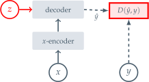
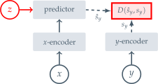
Imagine hiding several regions of a photograph and asking what belongs there. I-JEPA predicts a learned description of each hidden region, rather than its exact pixels. A context encoder sees only the visible patches; a predictor uses their features and target positions; a slowly updated target encoder supplies the training targets. Large target regions and a context spread across the image make the task require useful scene information. The learned encoder transfers to classification, counting and depth tasks. The experiments establish an effective image-pretraining recipe, rather than a complete predictive world model or a guarantee of human-like understanding.
1 Introduction
Pixel reconstruction spends effort on details that may not help recognition. View-invariance training can learn semantic features but relies on choices about which image changes should be ignored. I-JEPA instead predicts missing-region embeddings. Its contribution is the combination of representation-space targets, an asymmetric encoder–predictor design, and a masking strategy that makes semantic prediction useful. Comparisons cover frozen features, limited-label adaptation and local prediction tasks.
2 Background
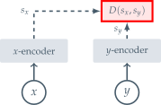
Self-supervision learns relationships within unlabeled data. In the energy-based view used here, compatible inputs should receive lower mismatch scores than incompatible ones. The following architectures differ in what they compare or predict.
Joint-Embedding Architectures.
A joint-embedding architecture makes two related image views have similar representations. Its obvious failure is collapse: every image receives the same vector. Contrastive examples, distributional regularization and asymmetric network updates are different ways of addressing that problem.
Generative Architectures.
A generative masked-image method predicts the hidden pixels or tokens themselves. Mask positions identify what must be reconstructed. This supplies a direct training target, but also requires modeling low-level details that may be irrelevant to a later task.
Joint-Embedding Predictive Architectures.
A JEPA predicts the representation of a target from the representation of its context, conditioned on information such as target position. Prediction replaces direct view matching, but collapse remains possible. I-JEPA uses a slowly updated target branch and a separate predictor; it does not derive a universal anti-collapse theorem.
3 Method
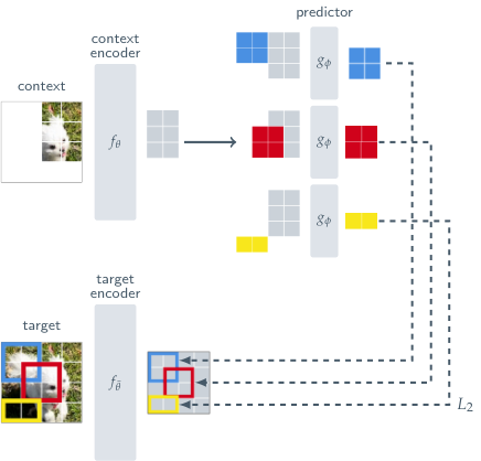
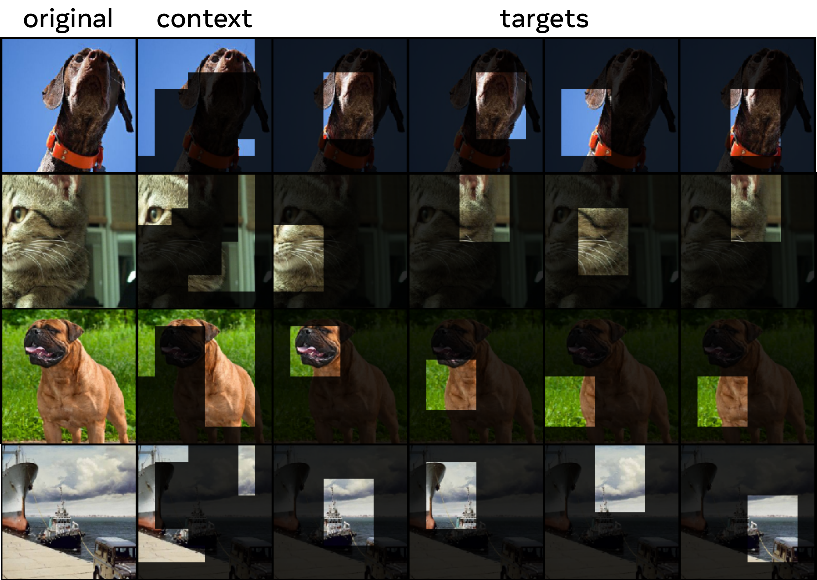
Three vision transformers share the work: a context encoder processes visible patches, a target encoder describes the full image, and a narrower predictor estimates selected target features. Figure 3 shows their connections; Figure 4 shows how masking removes overlap while leaving a distributed context.
Targets.
The target encoder first processes the complete image. Four blocks are then sampled from its output, each covering roughly 15–20% of the image with varying aspect ratio. Masking after encoding lets each target feature use full-image context, unlike encoding an isolated crop.
Context.
Start from a large context block covering 85–100% of the image, then remove every patch overlapping a target. The context encoder therefore receives a sparse collection of visible patches rather than the full image. Keeping enough distributed context makes the prediction task informative.
Prediction.
For each target block, the predictor combines visible-context features with learned mask tokens carrying the target locations. Running it separately for the four blocks produces a feature estimate for every requested target patch.
Loss.
Training minimizes squared feature error between predictions and target-encoder outputs. Gradients update the context encoder and predictor. The target encoder instead follows an exponential moving average of context-encoder weights, providing a slower-changing learning target.
Equation
4 Related Work
I-JEPA belongs to masked representation learning, alongside methods using pixels, discrete tokens or online feature targets. Its distinguishing goal is useful frozen semantic features without extensive handcrafted view augmentations. Data2vec and context autoencoders are particularly close comparisons; the retained table gives the actual pretraining and evaluation configurations.
| Method | Arch. | Epochs | Top-1 |
| Methods without view data augmentations | |||
| data2vec [8] | ViT-L/16 | 1600 | 77.3 |
| MAE [36] | ViT-B/16 | 1600 | 68.0 |
| ViT-L/16 | 1600 | 76.0 | |
| ViT-H/14 | 1600 | 77.2 | |
| CAE [22] | ViT-B/16 | 1600 | 70.4 |
| ViT-L/16 | 1600 | 78.1 | |
| I-JEPA | ViT-B/16 | 600 | 72.9 |
| ViT-L/16 | 600 | 77.5 | |
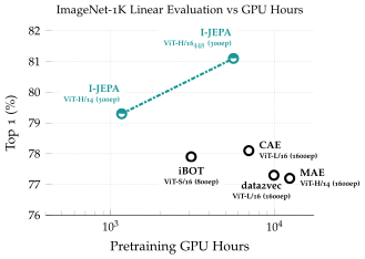
| ViT-H/14 | 300 | 79.3 | |
| ViT-H/ | 300 | 81.1 | |
| Methods using extra view data augmentations | |||
| SimCLR v2 [21] | RN152 () | 800 | 79.1 |
| DINO [18] | ViT-B/8 | 300 | 80.1 |
| iBOT [79] | ViT-L/16 | 250 | 81.0 |
5 Image Classification
Classification tests ask whether the pretrained features already organize images usefully. A frozen linear probe tests this directly; low-shot adaptation additionally tests whether a small labeled sample can make the representation useful.
| Method | Arch. | Epochs | Top-1 |
|---|---|---|---|
| Methods without view data augmentations | |||
| data2vec [8] | ViT-L/16 | 1600 | 73.3 |
| MAE [36] | ViT-L/16 | 1600 | 67.1 |
| ViT-H/14 | 1600 | 71.5 | |
| I-JEPA | ViT-L/16 | 600 | 69.4 |
| ViT-H/14 | 300 | 73.3 | |
| ViT-H/ | 300 | 77.3 | |
| Methods using extra view data augmentations | |||
| iBOT [79] | ViT-B/16 | 400 | 69.7 |
| DINO [18] | ViT-B/8 | 300 | 70.0 |
| SimCLR v2 [35] | RN151 () | 800 | 70.2 |
| BYOL [35] | RN200 () | 800 | 71.2 |
| MSN [4] | ViT-B/4 | 300 | 75.7 |
ImageNet-1K.
The encoder stays frozen while a linear classifier learns from ImageNet labels. I-JEPA improves on the compared pixel-reconstruction methods. Larger models and higher input resolution narrow the gap to augmentation-heavy joint-embedding methods; the headline scores compare different model sizes and training budgets.
Low-Shot ImageNet-1K.
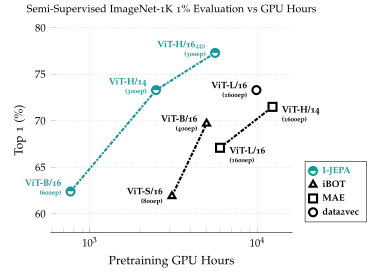
The 1%-label benchmark supplies only about 12–13 images per class. Each method uses its stronger adaptation protocol, either linear probing or fine-tuning. I-JEPA performs well in this setting, but those scores are not a uniform frozen-feature comparison across all methods.
Transfer learning.
Frozen features transfer to several image-classification datasets. I-JEPA improves over the compared non-augmentation methods and approaches the strongest view-invariance baselines, with performance depending on the dataset.
| Method | Arch. | CIFAR100 | Places205 | iNat18 |
|---|---|---|---|---|
| Methods without view data augmentations | ||||
| data2vec [8] | ViT-L/16 | 81.6 | 54.6 | 28.1 |
| MAE [36] | ViT-H/14 | 77.3 | 55.0 | 32.9 |
| I-JEPA | ViT-H/14 | 87.5 | 58.4 | 47.6 |
| Methods using extra view data augmentations | ||||
| DINO [18] | ViT-B/8 | 84.9 | 57.9 | 55.9 |
| iBOT [79] | ViT-L/16 | 88.3 | 60.4 | 57.3 |
6 Local Prediction Tasks
CLEVR counting and depth tasks probe information beyond image category. A linear model trained above a frozen encoder benefits from I-JEPA features relative to the tested view-invariance methods. These controlled tasks support the claim that the representation retains useful local structure.
| Method | Arch. | Clevr/Count | Clevr/Dist |
|---|---|---|---|
| Methods without view data augmentations | |||
| data2vec [8] | ViT-L/16 | 85.3 | 71.3 |
| MAE [36] | ViT-H/14 | 90.5 | 72.4 |
| I-JEPA | ViT-H/14 | 86.7 | 72.4 |
| Methods using extra data augmentations | |||
| DINO [18] | ViT-B/8 | 86.6 | 53.4 |
| iBOT [79] | ViT-L/16 | 85.7 | 62.8 |
| Pretrain | Arch. | CIFAR100 | Place205 | INat18 | Clevr/Count | Clevr/Dist |
|---|---|---|---|---|---|---|
| IN1k | ViT-H/14 | 87.5 | 58.4 | 47.6 | 86.7 | 72.4 |
| IN22k | ViT-H/14 | 89.5 | 57.8 | 50.5 | 88.6 | 75.0 |
| IN22k | ViT-G/16 | 89.5 | 59.1 | 55.3 | 86.7 | 73.0 |
7 Scalability
Model Efficiency.
Computing feature targets adds per-step cost relative to MAE, but the reported recipe needs many fewer training steps. The resulting compute savings are measured for these implementations and schedules. Processing one sparse context also avoids the multiple augmented views used by some baselines.
Scaling data size.
Pretraining on ImageNet-22K instead of ImageNet-1K improves both semantic and local downstream tasks in the reported comparisons. More diverse pretraining data is useful alongside the training objective.
Scaling model size.
Increasing model size improves several classification tasks. The largest model does not improve every local task: its larger input patches can discard spatial detail. Model capacity and spatial resolution therefore need separate consideration.
| Targets | Context | ||||
| Mask | Type | Freq. | Type | Avg. Ratio∗ | Top-1 |
| multi-block | Block | 4 | Block Complement | 0.25 | 54.2 |
| rasterized | Quadrant | 3 | Complement | 0.25 | 15.5 |
| block | Block | 1 | Complement | 0.4 | 20.2 |
| random | Random(0.6) | 1 | Complement | 0.4 | 17.6 |
| ∗Avg. Ratio is the average number of patches in the context block relative to the total number of patches in the image. | |||||
8 Predictor Visualizations
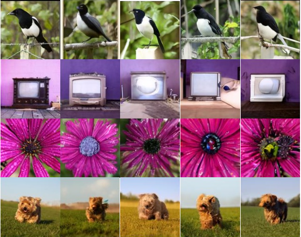
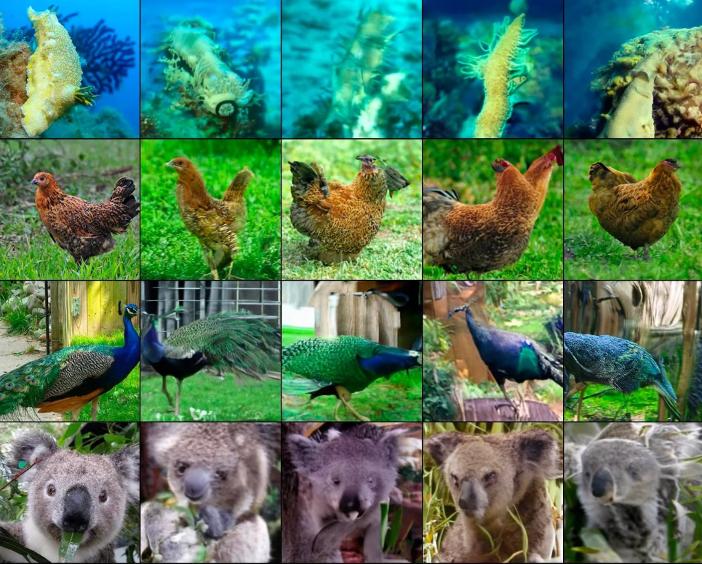
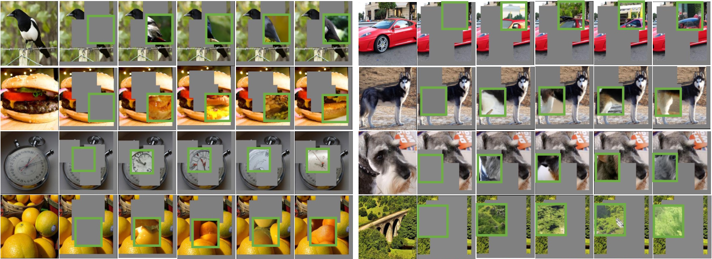
A separately trained conditional diffusion decoder turns predicted embeddings into illustrative images. Features shared across generated samples suggest information retained by the embedding; varying details suggest ambiguity. This visualization decoder is an analysis tool added after pretraining, not part of I-JEPA’s training objective.
9 Ablations
| Targets | Arch. | Epochs | Top-1 |
|---|---|---|---|
| Target-Encoder Output | ViT-L/16 | 500 | 66.9 |
| Pixels | ViT-L/16 | 800 | 40.7 |
Predicting in representation space.
Replacing learned feature targets with pixel targets reduces low-shot linear-probe performance in the tested ablation. This isolates evidence for representation-space prediction within the chosen training setup.
Masking strategy.
Multi-block targets outperform the compared random, single-block and quadrant strategies. The result concerns the combined information available in context and targets: simply hiding more pixels does not reproduce the successful recipe.
10 Conclusion
I-JEPA demonstrates efficient masked-feature pretraining with useful semantic and local image features. It is an image representation-learning result; downstream labels, task-specific probes and the chosen masking design remain part of its empirical story.
Appendix A Implementation Details
A.1 Pretraining
Architectures.
The predictor has width 384 and grows in depth with the encoder. Pretraining omits a classification token; evaluation averages target-encoder patch features. This distinguishes the representation being evaluated from a generic classification-token output.
Optimization.
AdamW trains the context encoder and predictor using a warmup and cosine learning-rate schedule. The default batch is 2048. Target-encoder averaging becomes progressively slower during training; the appendix specifies the learning-rate, weight-decay and momentum schedules.
Masking.
Four independently sampled target blocks overlap a large initial context mask; their overlap is removed from context. Equal token counts within each device’s batch make processing efficient. The data loader supplies masks as patch indices.
A.2 Downstream Tasks
Linear evaluation.
Frozen evaluation searches over the last layer or the last four layers and over alternative linear heads. I-JEPA uses pooled patch features where comparison methods may use classification tokens. Counting and depth avoid random cropping because it can remove the objects whose number or distance must be predicted.
ImageNet evaluations.
ImageNet linear probing follows a LARS-based recipe with a large batch and a small hyperparameter sweep. The encoder remains fixed, so this experiment measures information accessible through a shallow classifier.
Low-shot evaluation.
Low-shot evaluation fine-tunes the pretrained model for 50 epochs with AdamW, label smoothing and selected image augmentations. The absence of extensive view augmentations refers to pretraining; downstream adaptation still uses an explicitly chosen recipe.
Appendix B Broader Related Work
The broader discussion distinguishes information-maximizing regularization, architectural anti-collapse mechanisms and masked reconstruction. Maximizing retained information need not prefer task-relevant information over noise. I-JEPA’s position-conditioned predictor is a different local-prediction construction from contrastive patch discrimination.
Appendix C Additional Ablations
The extra ablations use a frozen linear probe on 1% of ImageNet labels. Their scores should be read separately from the main low-shot results that may use end-to-end fine-tuning.
Multiblock masking strategy.
Several sufficiently large target blocks and a broad initial context work best in these sweeps. Smaller contexts or fewer targets reduce accuracy, showing that the geometry of the prediction problem strongly affects learning.
| Targets | Context | ||
|---|---|---|---|
| Scale | Freq. | Scale | Top-1 |
| (0.075, 0.2) | 4 | (0.85, 1.0) | 19.2 |
| (0.1, 0.2) | 4 | (0.85, 1.0) | 39.2 |
| (0.125, 0.2) | 4 | (0.85, 1.0) | 42.4 |
| (0.15, 0.2) | 4 | (0.85, 1.0) | 54.2 |
| (0.2, 0.25) | 4 | (0.85, 1.0) | 38.9 |
| (0.2, 0.3) | 4 | (0.85, 1.0) | 33.6 |
| Targets | Context | ||
|---|---|---|---|
| Scale | Freq. | Scale | Top-1 |
| (0.15, 0.2) | 4 | (0.40, 1.0) | 31.2 |
| (0.15, 0.2) | 4 | (0.65, 1.0) | 47.1 |
| (0.15, 0.2) | 4 | (0.75, 1.0) | 49.3 |
| (0.15, 0.2) | 4 | (0.85, 1.0) | 54.2 |
| Targets | Context | ||
|---|---|---|---|
| Scale | Freq. | Scale | Top-1 |
| (0.15, 0.2) | 1 | (0.85, 1.0) | 9.0 |
| (0.15, 0.2) | 2 | (0.85, 1.0) | 22.0 |
| (0.15, 0.2) | 3 | (0.85, 1.0) | 48.5 |
| (0.15, 0.2) | 4 | (0.85, 1.0) | 54.2 |
Masking at the output of the target-encoder.
Selecting targets after full-image encoding outperforms separately encoding isolated target crops. The context available to the target encoder influences what its features ask the predictor to learn.
| Target Masking | Arch. | Epochs | Top-1 |
|---|---|---|---|
| Output | ViT-H/16 | 300 | 67.3 |
| Input | ViT-H/16 | 300 | 56.1 |
Predictor depth.
A 12-layer predictor improves the tested low-shot probe over a 6-layer predictor. This is a specific capacity ablation, not evidence that arbitrary additional depth always helps.
| Predictor Depth | Arch. | Epochs | Top-1 |
|---|---|---|---|
| 6 | ViT-L/16 | 500 | 64.0 |
| 12 | ViT-L/16 | 500 | 66.9 |
Weight decay.
Lower fixed weight decay improves low-shot fine-tuning but worsens full-label linear evaluation. The preferred pretraining recipe depends partly on which downstream protocol is valued.
| Weight Decay | Arch. | Epochs | ImageNet-1% | ImageNet Linear-Eval |
|---|---|---|---|---|
| ViT-L/16 | 600 | 69.4 | 77.8 | |
| ViT-L/16 | 600 | 70.7 | 76.4 |
Predictor width.
A narrow 384-channel predictor outperforms a 1024-channel predictor in the reported fine-tuning comparison. A bottleneck can improve learning rather than merely save computation.
| Predictor Width | Arch. | Epochs | Top-1 |
|---|---|---|---|
| 384 | ViT-L/16 | 600 | 70.7 |
| 1024 | ViT-L/16 | 600 | 68.4 |
Appendix D Finetuning on the full ImageNet
With full ImageNet fine-tuning, the high-resolution I-JEPA model reaches 87.1% top-1 accuracy, compared with 87.8% for the cited MAE configuration. Pretraining schedules differ substantially; the result demonstrates competitive adaptation rather than a matched-compute universal ranking.
Appendix E RCDM Visualizations
RCDM learns a separate diffusion decoder conditioned on frozen representation vectors. Sampling it with different noise seeds visualizes what those vectors constrain. Its training and generated images must not be mistaken for an image-generation capability trained inside I-JEPA.
E.1 Encoder Visualization
The I-JEPA visualizations tend to retain object identity, pose and layout while varying fine detail and background. The MSN comparison varies more of the object’s local structure. These examples are qualitative probes affected by a separately learned decoder, rather than direct reconstructions or definitive measurements of every represented feature.