Port-Hamiltonian neural networks (PHNNs) learn subsystem energy, dissipation, and input effects, then compose those models through a power-conserving interconnection. When the coupling is known, no composite-system training data are needed; when a constant coupling is unknown, a small regression problem estimates it. Numerical spring–mass–damper experiments demonstrate two-component and ten-component compositions. The evidence concerns state-observed simulated systems, not learned robot control or video observations.
1 Introduction
Learning one model per physical component can reduce the data needed to model new assemblies. The port-Hamiltonian structure supplies a common interface for combining learned and analytical components while maintaining energy-accounting properties. The paper provides training procedures, a composition rule, and a bound relating composite vector-field error to subsystem and coupling errors.
Figure 1:
An illustration of the compositional learning framework.
We train separate port-Hamiltonian neural networks (PHNNs) on data generated by individual subsystems, presented in §4.
We then compose these submodels to construct another PHNN that models the composite system, presented in §5.
2 Related Work
Neural differential equations and Hamiltonian models incorporate physical structure into learning. Port-Hamiltonian models additionally represent dissipation and external inputs. This work focuses on reusable composition of learned dynamics, whereas much previous work models a single system or learns controllers for already known dynamics. [4], [3], [27].
3 Port-Hamiltonian Systems
The state equation combines a skew-symmetric interconnection matrix, a positive-semidefinite dissipation matrix, the Hamiltonian gradient, and an input map. Skew symmetry conserves internal power; dissipation removes energy; the input–output pair accounts for supplied power. The formulation assumes finite-dimensional states without algebraic constraints.
Equation 1
(1)
3.1 An Illustrative Running Example: The Coupled Mass-Spring-Damper
Two separately modeled spring–mass–damper subsystems use spring elongation and momentum as state. Nonlinear damping is cubic in velocity. Their composite Hamiltonian is the sum of subsystem energies, while off-diagonal interconnection terms represent the force and motion coupling between the masses.
Figure 2:
An illustrative coupled spring-mass-damper example.
Two subsystems (left), with different spring and damping constants, are connected to obtain the composite system (right).
Equation 2
(2)
4 Port-Hamiltonian Neural Networks
Each subsystem learns only its unknown physical terms, then integrates the resulting differential equation to predict future states.
4.1 Constructing Port-Hamiltonian Neural Networks
A multilayer perceptron parameterizes energy, and automatic differentiation supplies its state gradient. Input maps may be constant parameters or state-dependent networks. Dissipation is represented as a matrix times its transpose to enforce positive semidefiniteness. Subsystem interconnection matrices are assumed known during this learning stage.
Figure 3:
An illustration of the construction and evaluation of a port-Hamiltonian Neural Network.
PHNNs enforce the cyclo-passivity property by construction.
Skew-symmetric interconnection and positive-semidefinite dissipation ensure that the modeled energy increase cannot exceed supplied input power. This is cyclo-passivity; the unconstrained learned Hamiltonian need not satisfy every additional condition required for an ordinary nonnegative storage function.
4.2 Evaluating Port-Hamiltonian Neural Networks
A PHNN predicts a future state by numerically integrating its learned vector field from the observed state. Solver accuracy and cost affect the result; all experiments use fixed-step fourth-order Runge–Kutta integration.
4.3 Training Port-Hamiltonian Neural Networks
Subsystem parameters are fitted by minimizing errors between integrated predictions and observed trajectory transitions. Training differentiates through the model evaluation and may include regularization; the reported experiments use no additional regularization.
Equation 3
(3)
5 Composing Port-Hamiltonian Neural Networks
Previously trained subsystem models are combined by assembling their physical terms, with only the inter-subsystem coupling supplied or learned separately.
5.1 Composing Models Using a Known Interconnection Structure
Composition sums subsystem Hamiltonians and places dissipation and input matrices on block diagonals. A skew-symmetric matrix with zero diagonal blocks adds cross-subsystem interactions. Each component energy must depend only on that component’s own state. The composite retains the structural energy-accounting properties.
5.2 Learning Compositions of Port-Hamiltonian Neural Network Submodels
Unknown coupling is learned while holding subsystem parameters fixed. A state-dependent coupling can use a neural parameterization; a constant skew-symmetric coupling gives linear equations from short-time transition data and can be fitted by least squares. The finite-difference approximation requires sufficiently small observation intervals.
Equation 4
(4)
5.3 Bounding the Errors of Composititions of Port-Hamiltonian Neural Networks
The stated theorem bounds composite vector-field error using subsystem dynamics errors, Hamiltonian-gradient errors, coupling-estimation errors, and coupling norms over prescribed domains. Known coupling removes the coupling-estimation term. This is a conditional error bound, not a guarantee that arbitrary learned energies or long rollout errors are small.
Equation 5
(5)
6 Numerical Experiments
Numerical experiments study nonlinear spring–mass–damper systems with external forcing, using either known or estimated couplings.
6.1 Composing Port-Hamiltonian Neural Networks Using a Known Composition Term
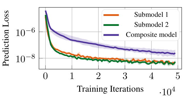
Each of two subsystem models trains on 100 trajectories. Composite predictions use their learned components without composite training data. Plots report median errors and interquartile ranges over ten independent runs, using 20 held-out trajectories per test set.
Figure 4:
Prediction loss values throughout training.
The composite model makes accurate predictions without any training data from the composite system itself.
The composite model accurately predicts dynamics without data from the composite system.
Composite prediction error decreases alongside subsystem training error in the reported experiment. The blue curve is evaluation of a composition, not a separately trained composite model. No monolithic baseline is trained in this no-composite-data setting.
6.2 Learning the Interactions Between Subsystem Port-Hamiltonian Neural Networks
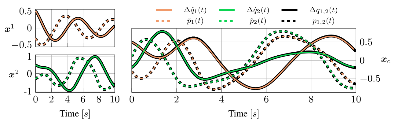
With subsystem models already trained, four single-step transitions from random composite states are used to estimate a constant interconnection by least squares. The resulting trajectories track the numerical ground truth closely in the illustrated test.
Figure 5:
The composite PHNN accurately predicts state trajectories, even when the unknown composition term is inferred using only four transition datapoints.
Left: Predicted subsystem dynamics.
Right: Predicted composite system dynamics.
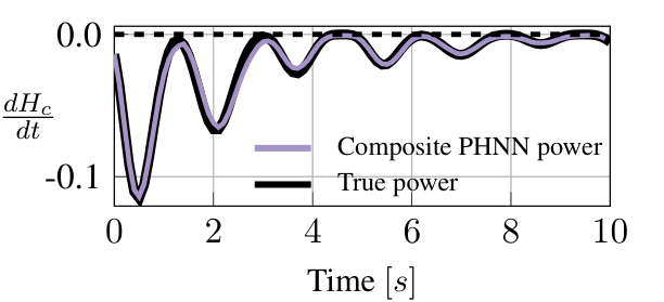
Figure 6: Time derivative of the system’s Hamiltonian with no external control inputs.
We accurately learn the unknown composition term using a negligible amount of data.
The four-transition result demonstrates economical identification for this small, structured coupling problem. It does not mean the full subsystem dynamics were learned from four data points.
The learned composite model enjoys properties of port-Hamiltonian systems.
Without external forcing, the plotted learned Hamiltonian derivative remains nonpositive along the tested trajectory, consistent with the model’s structural cyclo-passivity.
6.3 Predicting the Dynamics of Ten Interacting Subsystems Without Additional Training
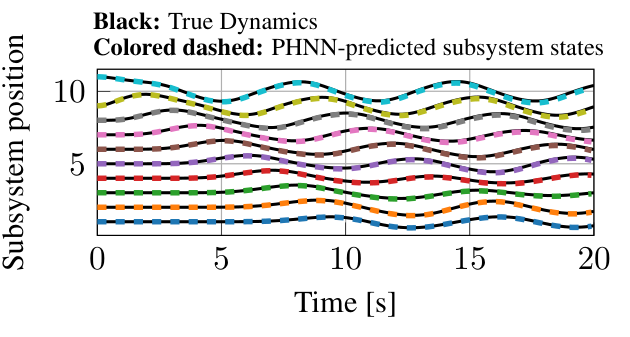
Reusing the two learned subsystem types in a ten-component chain predicts wave-like energy propagation under sinusoidal forcing. Neither subsystem retraining nor ten-component trajectory data are used; the new assembly’s coupling structure is supplied.
Figure 7: The composite PHNN accurately predicts the dynamics of interacting subsystems with no additional training.
7 Conclusions
Physics-informed interfaces enable modular reuse and compositions requiring little or no additional system data. Learning from video and using the composed models for feedback control are proposed next steps. The experiments are limited to numerical spring–mass–damper systems.
Appendix A Proof of Theorem 1
The proof separates total error into uncoupled subsystem error and an interaction term. Triangle inequalities and operator norms then bound coupling mismatch and Hamiltonian-gradient mismatch, giving the stated composite vector-field bound. The complete algebra is retained below.
Equations 6–19
(6)
(7)
(8)
(9)
(10)
(11)
(12)
(13)
(14)
(15)
(16)
(17)
(18)
(19)
Appendix B Additional Experimental Details
The supplement specifies simulation generation, network sizes, optimization, and hardware.
B.1 Simulation Details
Fourth-order Runge–Kutta simulation uses a 0.01-second step. Each training set has 100 trajectories of 500 steps, with initial elongations and momenta sampled from bounded intervals; test sets contain 20 trajectories. Sinusoidal inputs excite the controlled subsystem and composite system. The source’s second damping-parameter entry is malformed, so the explicit matrices and supplied code are preferable for exact reproduction.
Equations 20–21
(20)
(21)
B.2 Neural Network Implementations
Energy and dissipation networks use two hidden layers of 32 tanh units; constant input-matrix entries are learned directly. JAX supplies differentiation and compilation. Adam uses learning rate 0.001 and minibatches of 32, with no additional loss regularization.
39 references
Bradbury et al. (2018)
James Bradbury, Roy Frostig, Peter Hawkins, Matthew James Johnson, Chris Leary,
Dougal Maclaurin, George Necula, Adam Paszke, Jake VanderPlas, Skye
Wanderman-Milne, and Qiao Zhang.
JAX: composable transformations of Python+NumPy programs,
2018.
URLhttp://github.com/google/jax.
Cardoso-Ribeiro et al. (2015)
Flávio Luiz Cardoso-Ribeiro, Denis Matignon, and Valérie Pommier-Budinger.
Modeling of a fluid-structure coupled system using port-hamiltonian
formulation.
IFAC-PapersOnLine, 48(13):217–222, 2015.
Chen et al. (2018)
Ricky T. Q. Chen, Yulia Rubanova, Jesse Bettencourt, and David K Duvenaud.
Neural ordinary differential equations.
In Advances in Neural Information Processing Systems,
volume 31, 2018.
Cherifi et al. (2019)
Karim Cherifi, Volker Mehrmann, and Kamel Hariche.
Numerical methods to compute a minimal realization of a
port-hamiltonian system.
arXiv:1903.07042, 2019.
Cherifi et al. (2022)
Karim Cherifi, Pawan Kumar Goyal, and Peter Benner.
A non-intrusive method to inferring linear port-hamiltonian
realizations using time-domain data.
Electronic Transactions on Numerical Analysis: Special Issue
SciML, 56:102–116, 2022.
Cranmer et al. (2020)
Miles Cranmer, Sam Greydanus, Stephan Hoyer, Peter Battaglia, David Spergel,
and Shirley Ho.
Lagrangian neural networks.
In Workshop on Integration of Deep Neural Models and
Differential Equations, International Conference on Learning
Representations, 2020.
Dai et al. (2019)
Siyuan Dai, Zhenkai Zhang, and Xenofon Koutsoukos.
A model-based design approach for simulation and virtual prototyping
of automotive control systems using port-hamiltonian systems.
Software & Systems Modeling, 18(3):1637–1653, 2019.
Desai et al. (2021)
Shaan A Desai, Marios Mattheakis, David Sondak, Pavlos Protopapas, and
Stephen J Roberts.
Port-hamiltonian neural networks for learning explicit time-dependent
dynamical systems.
Physical Review E, 104(3):034312, 2021.
Djeumou et al. (2022a)
Franck Djeumou, Cyrus Neary, Eric Goubault, Sylvie Putot, and Ufuk Topcu.
Neural networks with physics-informed architectures and constraints
for dynamical systems modeling.
In Proceedings of The 4th Annual Learning for Dynamics and
Control Conference, volume 168 of Proceedings of Machine Learning
Research, 2022a.
Djeumou et al. (2022b)
Franck Djeumou, Cyrus Neary, Eric Goubault, Sylvie Putot, and Ufuk Topcu.
Taylor-lagrange neural ordinary differential equations: Toward fast
training and evaluation of neural odes.
In Proceedings of the 31st International Joint Conference on
Artificial Intelligence, 2022b.
Donaire and Junco (2009)
Alejandro Donaire and Sergio Junco.
Derivation of input-state-output port-hamiltonian systems from bond
graphs.
Simulation Modelling Practice and Theory, 17(1):137–151, 2009.
Duindam et al. (2009)
Vincent Duindam, Alessandro Macchelli, Stefano Stramigioli, and Herman
Bruyninckx.
Modeling and control of complex physical systems: the
port-Hamiltonian approach.
Springer Science & Business Media, 2009.
Duong and Atanasov (2021)
Thai Duong and Nikolay Atanasov.
Hamiltonian-based neural ode networks on the se (3) manifold for
dynamics learning and control.
In Proceedings of Robotics: Science and Systems, 2021.
Finzi et al. (2020)
Marc Finzi, Ke Alexander Wang, and Andrew G Wilson.
Simplifying hamiltonian and lagrangian neural networks via explicit
constraints.
In Advances in Neural Information Processing Systems,
volume 33, 2020.
Furieri et al. (2022)
Luca Furieri, Clara Lucía Galimberti, Muhammad Zakwan, and Giancarlo
Ferrari-Trecate.
Distributed neural network control with dependability guarantees: a
compositional port-hamiltonian approach.
In Proceedings of The 4th Annual Learning for Dynamics and
Control Conference, volume 168 of Proceedings of Machine Learning
Research, 2022.
Greydanus et al. (2019)
Samuel Greydanus, Misko Dzamba, and Jason Yosinski.
Hamiltonian neural networks.
In Advances in Neural Information Processing Systems,
volume 32, 2019.
Gupta et al. (2020)
Jayesh K. Gupta, Kunal Menda, Zachary Manchester, and Mykel Kochenderfer.
Structured mechanical models for robot learning and control.
In Proceedings of the 2nd Conference on Learning for Dynamics
and Control, volume 120 of Proceedings of Machine Learning Research,
2020.
Lopes et al. (2015)
Nicolas Lopes, Thomas Hélie, and Antoine Falaize.
Explicit second-order accurate method for the passive guaranteed
simulation of port-hamiltonian systems.
IFAC-PapersOnLine, 48(13):223–228, 2015.
Lutter et al. (2019)
Michael Lutter, Christian Ritter, and Jan Peters.
Deep lagrangian networks: Using physics as model prior for deep
learning.
In International Conference on Learning Representations, 2019.
Matsubara et al. (2020)
Takashi Matsubara, Ai Ishikawa, and Takaharu Yaguchi.
Deep energy-based modeling of discrete-time physics.
In Advances in Neural Information Processing Systems,
volume 33, 2020.
Menda et al. (2019)
Kunal Menda, Jayesh K Gupta, Zachary Manchester, and Mykel J Kochenderfer.
Structured mechanical models for efficient reinforcement learning.
In Workshop on Structure and Priors in Reinforcement Learning,
International Conference on Learning Representations, 2019.
Nageshrao et al. (2016)
Subramanya P. Nageshrao, Gabriel A. D. Lopes, Dimitri Jeltsema, and Robert
Babuška.
Port-hamiltonian systems in adaptive and learning control: A survey.
IEEE Transactions on Automatic Control, 61(5):1223–1238, 2016.
Plaza et al. (2022)
Santiago Sanchez-Escalonilla Plaza, Rodolfo Reyes-Báez, and Bayu
Jayawardhana.
Total energy shaping with neural interconnection and damping
assignment - passivity based control.
In Proceedings of The 4th Annual Learning for Dynamics and
Control Conference, volume 168 of Proceedings of Machine Learning
Research, 2022.
Rackauckas et al. (2020)
Christopher Rackauckas, Yingbo Ma, Julius Martensen, Collin Warner, Kirill
Zubov, Rohit Supekar, Dominic Skinner, Ali Ramadhan, and Alan Edelman.
Universal differential equations for scientific machine learning.
arXiv:2001.04385, 2020.
Rashad et al. (2022)
Ramy Rashad, Davide Bicego, Jelle Zult, Santiago Sanchez-Escalonilla, Ran Jiao,
Antonio Franchi, and Stefano Stramigioli.
Energy aware impedance control of a flying end-effector in the
port-hamiltonian framework.
IEEE Transactions on Robotics, 38(6):3936–3955, 2022.
Roehrl et al. (2020)
Manuel A Roehrl, Thomas A Runkler, Veronika Brandtstetter, Michel Tokic, and
Stefan Obermayer.
Modeling system dynamics with physics-informed neural networks based
on lagrangian mechanics.
IFAC-PapersOnLine, 53(2):9195–9200, 2020.
Shi et al. (2019)
Guanya Shi, Xichen Shi, Michael O’Connell, Rose Yu, Kamyar Azizzadenesheli,
Animashree Anandkumar, Yisong Yue, and Soon-Jo Chung.
Neural lander: Stable drone landing control using learned dynamics.
In International Conference on Robotics and Automation, 2019.
Strehle et al. (2018)
Felix Strehle, Martin Pfeifer, Lukas Kölsch, Charlotte Degünther,
Johannes Ruf, Lisa Andresen, and Sören Hohmann.
Towards port-hamiltonian modeling of multi-carrier energy systems: A
case study for a coupled electricity and gas distribution system.
IFAC-PapersOnLine, 51(2):463–468, 2018.
Toth et al. (2020)
Peter Toth, Danilo J. Rezende, Andrew Jaegle, Sébastien Racanière,
Aleksandar Botev, and Irina Higgins.
Hamiltonian generative networks.
In International Conference on Learning Representations, 2020.
Van Der Schaft (2020)
Arjan Van Der Schaft.
Port-hamiltonian modeling for control.
Annual Review of Control, Robotics, and Autonomous Systems,
3(1):393–416, 2020.
Van Der Schaft et al. (2014)
Arjan Van Der Schaft, Dimitri Jeltsema, et al.
Port-hamiltonian systems theory: An introductory overview.
Foundations and Trends in Systems and Control, 1(2-3):173–378, 2014.
Zhong et al. (2020)
Yaofeng Desmond Zhong, Biswadip Dey, and Amit Chakraborty.
Dissipative symODEN: Encoding hamiltonian dynamics with dissipation
and control into deep learning.
In Workshop on Integration of Deep Neural Models and
Differential Equations, International Conference on Learning
Representations, 2020.
Zhong et al. (2021a)
Yaofeng Desmond Zhong, Biswadip Dey, and Amit Chakraborty.
Benchmarking energy-conserving neural networks for learning dynamics
from data.
In Proceedings of the 3rd Conference on Learning for Dynamics
and Control, volume 144 of Proceedings of Machine Learning Research,
2021a.
Zhong et al. (2021b)
Yaofeng Desmond Zhong, Biswadip Dey, and Amit Chakraborty.
Extending lagrangian and hamiltonian neural networks with
differentiable contact models.
In Advances in Neural Information Processing Systems,
volume 34, 2021b.