At a glance
Intuition. A camera watches a moving dot against a textured wall. Predicting tomorrow’s wall texture can be easier than tracking the dot. This early JEPA study shows why “predictable” and “useful” are different requirements: a representation can satisfy its self-supervised objective while discarding the object a later task needs.
The authors compare two embedding-prediction losses with pixel reconstruction and inverse dynamics in controlled offline environments. Changing distractors are handled well; fixed distractors expose a failure. These are toy-environment findings, not a measurement of every later JEPA model.
1 Introduction
The paper tests whether reconstruction-free world models learn useful state information without reward labels. Rather than score the pretraining loss alone, it asks a separately trained probe to recover a moving dot’s position from the learned state and its predicted future states. Static and changing backgrounds separate easy temporal consistency from useful dynamics.
2 Method
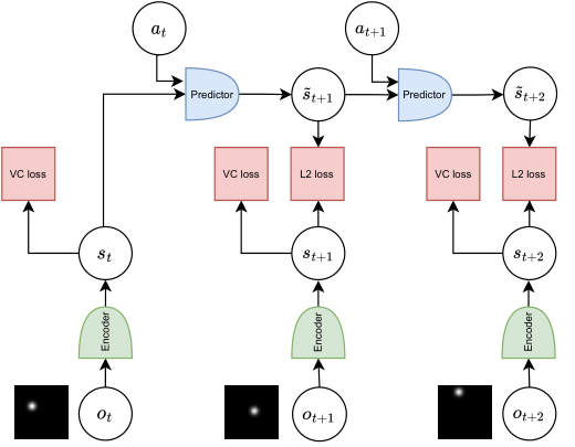
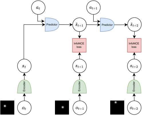
An encoder maps each image to a state vector. An action-conditioned predictor rolls that vector forward repeatedly, starting from the first image rather than re-encoding every future observation. A frozen model is evaluated by fitting a linear position readout. The two JEPA variants use VICReg or SimCLR to match predictions to encoded future observations. Reconstruction additionally decodes images; inverse dynamics predicts actions between observed states. Supervised and random encoders provide reference points. All methods share encoder/predictor architectures, receive no image augmentations and are trained through the rollout, making the loss choice a central experimental difference.
2.1 Spurious correlation
A fixed background offers a shortcut: encode its random pixel values and predict the same vector forever. Different episodes still contain different backgrounds, so the embeddings can vary across the batch while ignoring motion within each episode. Under the stated construction, this can satisfy VICReg’s prediction, variance and decorrelation terms. The contrastive analogue also rewards matching the same background across time. Avoiding one identical vector for every input therefore does not ensure that the learned representation preserves the task-relevant object.
Equations 1–4
| (1) |
| (2) |
| (3) | ||||
| (4) |
3 Experiments
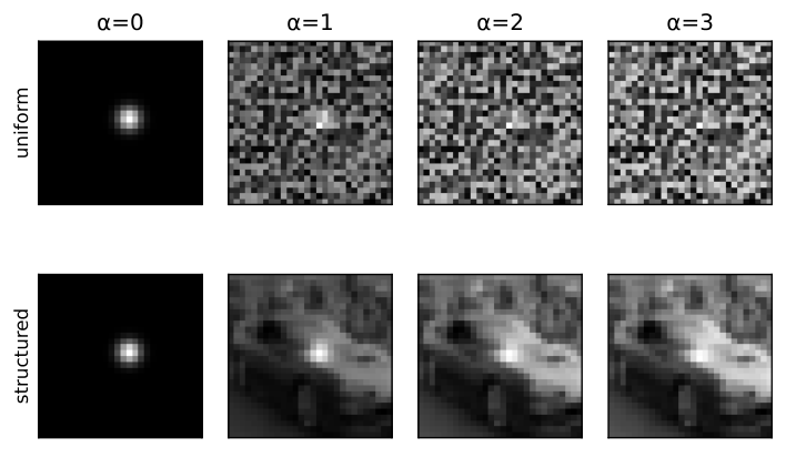
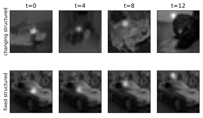
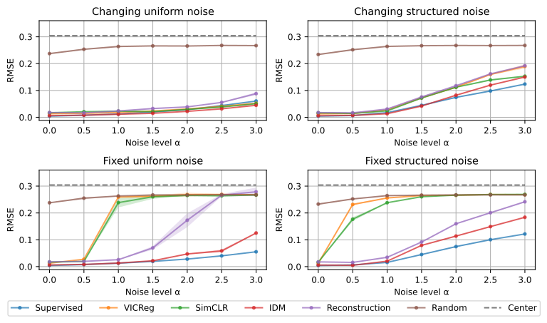
Each sequence contains 17 images and 16 displacement actions for one dot in a bounded square. Pretraining uses one million sequences; a separate position probe uses 300,000, with 10,000 evaluation sequences. Distractors are either uniform random patterns or CIFAR-10 images. They are resampled every frame or held fixed within an episode, and their brightness is varied. Hyperparameters are tuned separately by condition.
3.1 Results
With no distractors, all methods work well. With frame-changing noise, the embedding methods remain useful and need less retuning than reconstruction in some conditions. Fixed noise reverses the advantage: both tested JEPA losses fail to retain the moving dot’s location. Inverse dynamics handles the controlled object, but its success has a different blind spot: it can ignore useful things unaffected by the agent. The three-dot experiment in the appendix makes that tradeoff visible.
4 Conclusion
The practical lesson is to inspect what a predictor preserves, rather than assuming temporal predictability selects useful state variables. The authors suggest hierarchy or constraints that require change across time, but do not establish a general fix here. Inputs such as optical flow may remove some static shortcuts while also removing useful static context. Later JEPA objectives and architectures should be evaluated on their own evidence rather than inheriting either this failure or a promise of immunity.
Checklist
The checklist locates code, implementation details, hyperparameter searches, uncertainty reporting and compute information in the appendix. No human-subject study or newly collected personal dataset is involved. Its purpose is reproducibility and disclosure; it does not add an independent performance result.
Appendix A Appendix
A.1 Related work
Joint Embedding methods
Joint-embedding image methods motivate the tested losses. Prior work already notes that easy shared features can dominate contrastive training; this study isolates how that concern appears in action-conditioned video prediction.
Representation learning from video
Earlier video representation methods use time-linked positives and several kinds of negatives. Their training tasks and sampling rules differ, so the present counterexample concerns the particular forward-model objectives implemented here.
Forward model learning
Generative world models reconstruct observations, while other work learns contrastive or reward-equivalent states. This paper assumes the future evaluation reward is unknown, and explicitly includes distractors that remain fixed through time.
Self-supervised learning for reinforcement learning
Self-supervised pretraining can improve reinforcement-learning encoders. This evaluation additionally tests the predicted latent rollout, not just the representation computed directly from an observed image.
A.2 Dataset
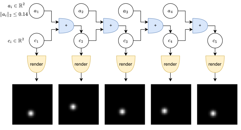
Images are 28 × 28, and a dot moves by a bounded two-dimensional displacement with clipping at the square’s edge. Each episode samples a preferred motion direction, then varied step directions and lengths; this avoids a trajectory that simply stays near its starting point in expectation. Gaussian blurring renders the dot. Uniform noise or CIFAR-10 imagery is added with a brightness coefficient, either fixed within an episode or independently changing at each step. Thus the experiment controls temporal persistence separately from visual complexity.
A.3 Training methods details
For each minibatch, the encoder produces observed states and the recurrent predictor produces an action-conditioned rollout from the initial state. The appendix writes each loss on these aligned sequences. Shared symbols and rollout lengths matter when reproducing the comparisons.
A.3.1 VICReg
VICReg matches predicted and observed states while penalizing insufficient variance and redundant coordinates at each time step. Batch diversity prevents a universal constant representation, but permits the static-background shortcut described earlier.
Equations 5–9
| (5) | ||||
| (6) | ||||
| (7) | ||||
| (8) | ||||
| (9) |
A.3.2 SimCLR
The SimCLR adaptation treats a prediction and its corresponding encoded future observation as a positive pair. Its contrastive loss is applied separately at each rollout time; other examples supply negatives.
Equations 10–12
| (10) | ||||
| (11) | ||||
| (12) |
A.3.3 Inverse Dynamics Modeling (IDM)
Inverse dynamics predicts the intervening action from consecutive encoded observations. This steers the encoder toward controllable changes, while the forward predictor still matches the next observed latent state. It need not preserve unrelated static context.
Equations 13–15
| (13) | ||||
| (14) | ||||
| (15) |
A.3.4 Reconstruction
The reconstruction baseline decodes predicted states back into images and minimizes pixel error. Its decoder mirrors the encoder with upsampling. This objective retains visual detail that latent-prediction losses can choose to discard.
Equation 16
| (16) |
A.4 Probing details
The position probe is a single linear layer trained with encoder and predictor frozen. It reads both the first encoded state and later action-conditioned predicted states. Errors therefore test whether position remains linearly accessible across a rollout, not whether a powerful new decoder could recover it after additional end-to-end training.
Equation 18
| (18) |
A.5 Additional results
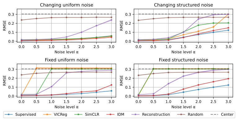
The additional curves hold noise-free hyperparameters fixed across distractor strengths. This distinguishes robustness without retuning from the tuned main comparison. Reconstruction degrades under changing uniform noise; the JEPA variants still fail with sufficiently strong fixed distractions.
A.6 3 dots dataset
A.6.1 Environment
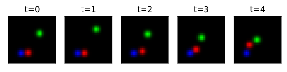
A second environment contains three separately identifiable dots: one controlled by supplied actions, one moving unpredictably and one stationary within an episode. The desired state retains the controlled and stationary dots while ignoring the unpredictable one.
A.6.2 Results
The tested JEPA losses favor the stationary dot and lose the other two. Inverse dynamics retains the controlled dot but misses the stationary one. Reconstruction captures both predictable dots. This separates the objectives’ preferences rather than identifying one method that is best for every possible downstream task.
| Method | Average | Action | Random | Stationary |
|---|---|---|---|---|
| VICReg | 0.229±0.031 | 0.277±0.041 | 0.273±0.044 | 0.066±0.026 |
| SimCLR | 0.158±0.001 | 0.193±0.001 | 0.193±0.002 | 0.025±0.001 |
| IDM | 0.234±0.001 | 0.035±0.000 | 0.298±0.002 | 0.272±0.000 |
| Supervised | 0.104±0.000 | 0.010±0.001 | 0.180±0.001 | 0.005±0.000 |
| Reconstruction | 0.107±0.000 | 0.021±0.001 | 0.182±0.000 | 0.026±0.002 |
| Random | 0.260±0.001 | 0.235±0.002 | 0.278±0.002 | 0.265±0.004 |
| Center | 0.299±0.000 | 0.304±0.000 | 0.304±0.000 | 0.289±0.000 |
A.7 Model architectures
The encoder uses three convolutional layers with normalization, nonlinearities and pooling, followed by a 512-dimensional output. A single-layer gated recurrent unit predicts future states from actions. The reconstruction decoder reverses the spatial reduction. This implementation uses no additional latent variable for alternative futures.
A.8 Limitations
The results come from simple synthetic environments and only two JEPA losses. They identify a concrete possible failure, without establishing its prevalence in large natural-video models or in newer collapse-prevention objectives.
A.9 Computational resources
Experiments use AMD MI50 or Nvidia RTX 8000 accelerators. For each distractor type and strength, 100 hyperparameter choices are searched; the best setting is repeated for three seeds. A single run takes less than one accelerator-hour.
A.10 Code license
Parts of the reconstruction and contrastive implementations reuse MIT-licensed code. The source identifies the relevant upstream implementations.
A.11 Acknowledgements
The work acknowledges National Science Foundation support.