Literature
Display
← All papers

Engineering Monosemanticity in Toy Models

Adam S. Jermyn · Nicholas Schiefer · Evan Hubinger

· arXiv (preprint) ↗

Interpretability5 min text · CondensedOriginal paper ↗
Contents

At a glance

Negative bias initialization can steer small networks toward more interpretable neurons without worsening loss in several controlled sparse-feature settings. Wider hidden layers also help, at higher compute cost. The result is task-dependent: absolute-value models need a slower bias-decay schedule, and the study does not establish the same tradeoff for language models. [2]

1 Introduction

The paper separates the motivation for interpretable neurons from experiments in which useful input features are known exactly.

1.1 Motivation

A neuron is easier to interpret when it responds to one useful feature rather than an unrelated mixture. These experiments ask whether training choices can favor that organization without sacrificing task performance.

1.2 Overview

Two learned linear maps surround a nonlinear hidden layer. Three synthetic tasks separate input dimension, number of possible features, and number of nonlinear units. The study compares loss basins, tests negative biases and width, then analyzes the most monosemantic feature-decoder models.
Refer to caption
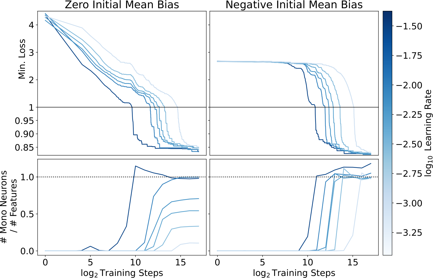
Figure 1: Models initialized with zero mean bias (left, batch LR1) find different local minima depending on the learning rate, with more monosemantic solutions and slightly lower loss at higher learning rates. Models initialized with a negative mean bias (right, batch LR3) all find highly monosemantic local minima, and achieve slightly better loss.

2 Setup

The synthetic data, three target tasks, and adjustable-width architecture define the controlled setting used throughout.

2.1 Features

Each of 512 possible features is usually zero and otherwise uniform on [0,1]. Feature occurrence is either equally frequent or follows a power law proportional to rank raised to −1.1. A fixed random projection compresses these sparse feature vectors into fewer dimensions.

2.2 Tasks

The tasks are feature recovery, conversion between random projections, and recovery of absolute feature values. Knowing the generating features makes neuron selectivity measurable.

2.2.1 Feature Decoder

The decoder reconstructs the original feature vector from its fixed lower-dimensional random projection using squared-error loss. Recovery depends on the input’s sparsity and projection, rather than being possible for arbitrary dense vectors.

Equation 1
L=||f→−y→||2,\displaystyle L=\left|\left|\vec{f}-\vec{y}\right|\right|^{2}, (1)

2.2.2 Re-Projector

The re-projector predicts a second fixed random projection from the first. This changes the output basis while retaining the same underlying sparse-feature structure.

Equation 2
L=|Q⋅f→−y→|2.\displaystyle L=\left|Q\cdot\vec{f}-\vec{y}\right|^{2}. (2)

2.2.3 Absolute Value Calculator

The absolute-value task projects the difference of two independently sampled feature vectors, then predicts its elementwise absolute value. It requires both recovering information and applying a nonlinear transformation.

Equation 3
L=|||f|→−y→||2,\displaystyle L=\left|\left|\vec{|f|}-\vec{y}\right|\right|^{2}, (3)

2.3 Architecture

A biased linear encoder feeds ReLU or GeLU units, followed by an unbiased linear output layer. Hidden width varies independently of input and feature dimensions, unlike a tied-width reconstruction model.

Equations 4–6
e→\displaystyle\vec{e} =L1⋅x→+b→,\displaystyle=L_{1}\cdot\vec{x}+\vec{b}, (4)
h→\displaystyle\vec{h} =N⁡[e→],\displaystyle=N[\vec{e}], (5)
y→\displaystyle\vec{y} =L2⋅h→.\displaystyle=L_{2}\cdot\vec{h}. (6)

3 Measuring Monosemanticity

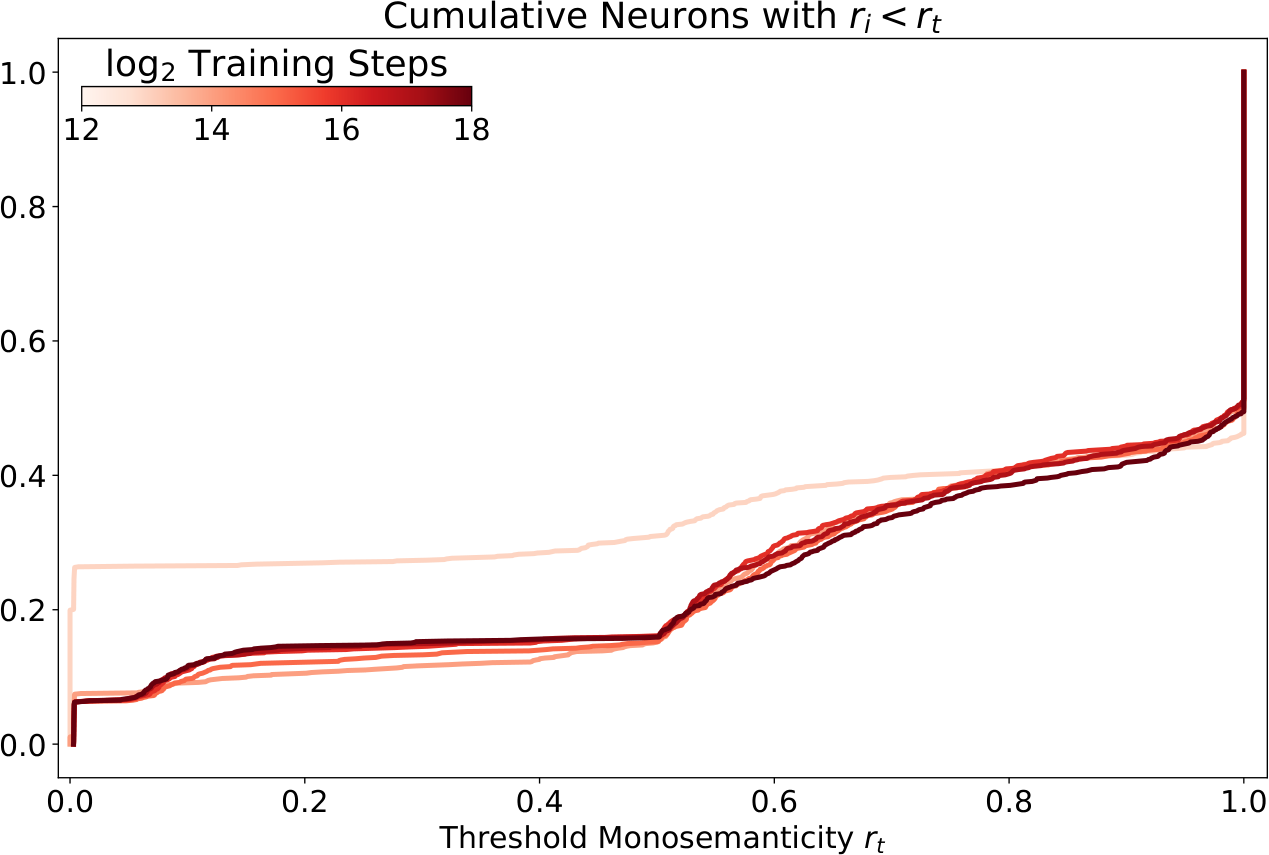
The selectivity score divides a neuron’s largest positive response to any unit-strength single-feature input by its summed positive responses. The paper labels scores above 0.999 monosemantic, adapting the test for signed inputs in the absolute-value task. This diagnostic examines controlled single-feature probes, not all possible feature mixtures.

Equation 7
ri≡maxj⁡(hi​(Fj))δ+∑jmax⁡(0,hi​(Fj)),\displaystyle r_{i}\equiv\frac{\max_{j}(h_{i}(F_{j}))}{\delta+\sum_{j}\max(0,h_{i}(F_{j}))}, (7)
Refer to caption
Figure 2: The cumulative fraction of neurons with monosemanticity ri<rtr_{i}<r_{t} for varying thresholds rtr_{t} for a model from batch K1 with 1024 neurons. The sharp spike at rt=1r_{t}=1 reflects a population of precisely monosemantic neurons.

4 Results

Default experiments use 512 features, 64 input dimensions, feature frequency 1/64, and thus eight active features on average. Many decoder runs achieve similar loss with substantially different selectivity. Negative biases and sufficient width favor interpretable units, but all three tasks do not share an identical loss–interpretability tradeoff.

4.1 Task: Feature Decoder

The feature-decoder experiments examine optimization basins, bias initialization, activation regularization, hidden width, and feature sparsity separately.

4.1.1 Monosemantic and Polysemantic Basins

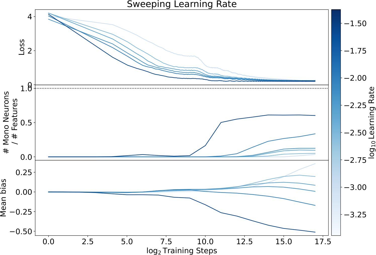
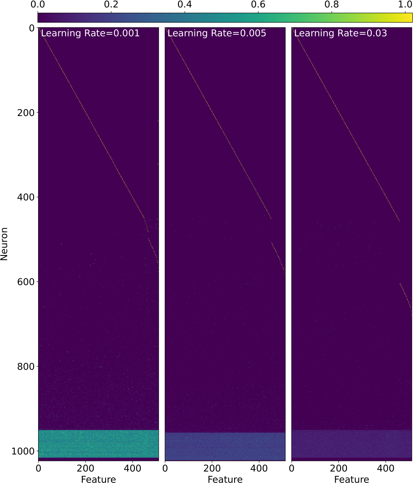
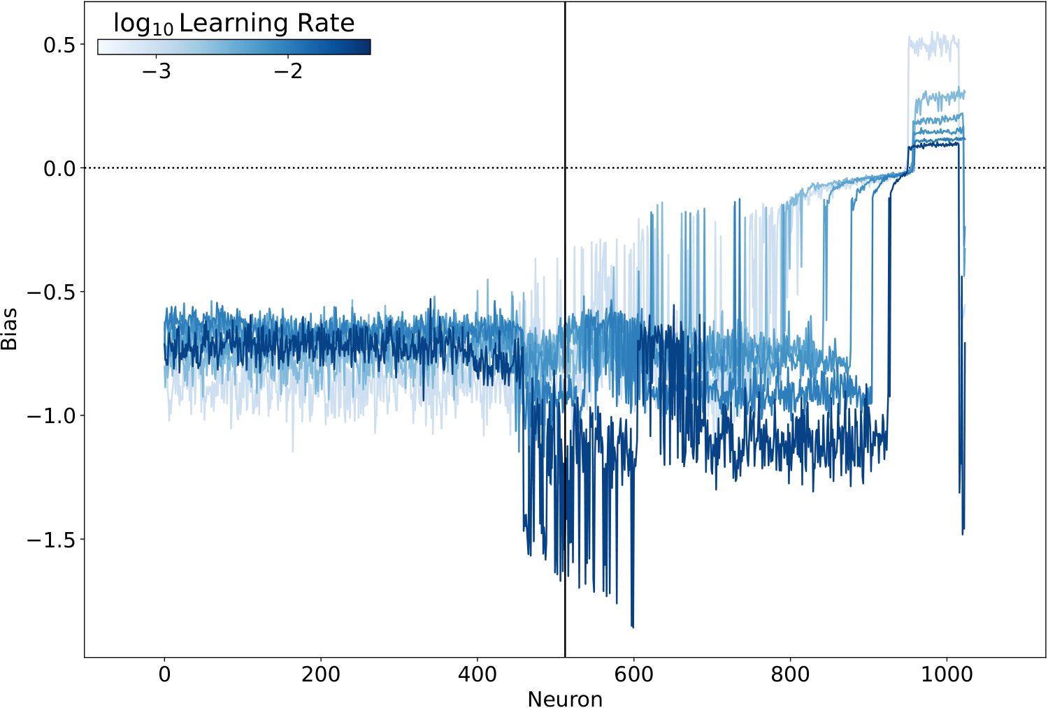
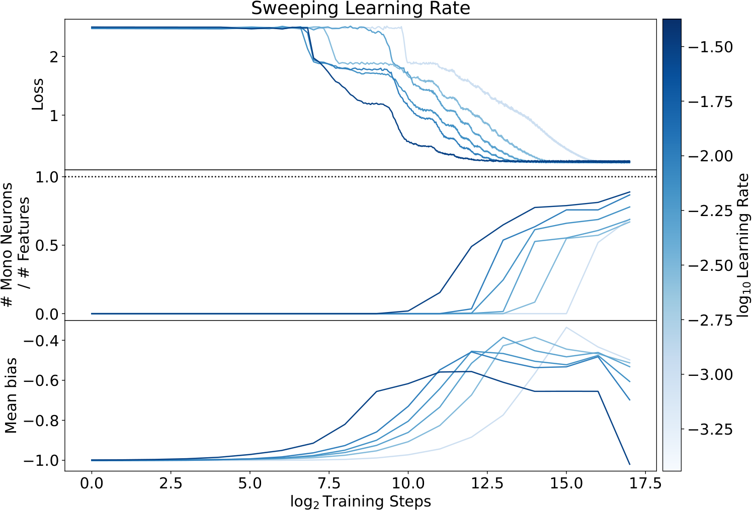
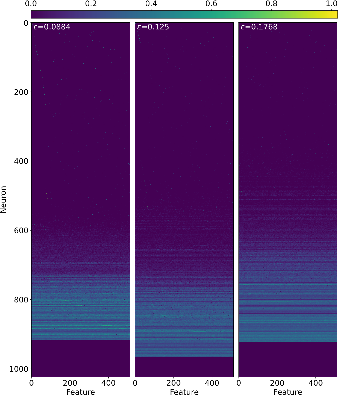
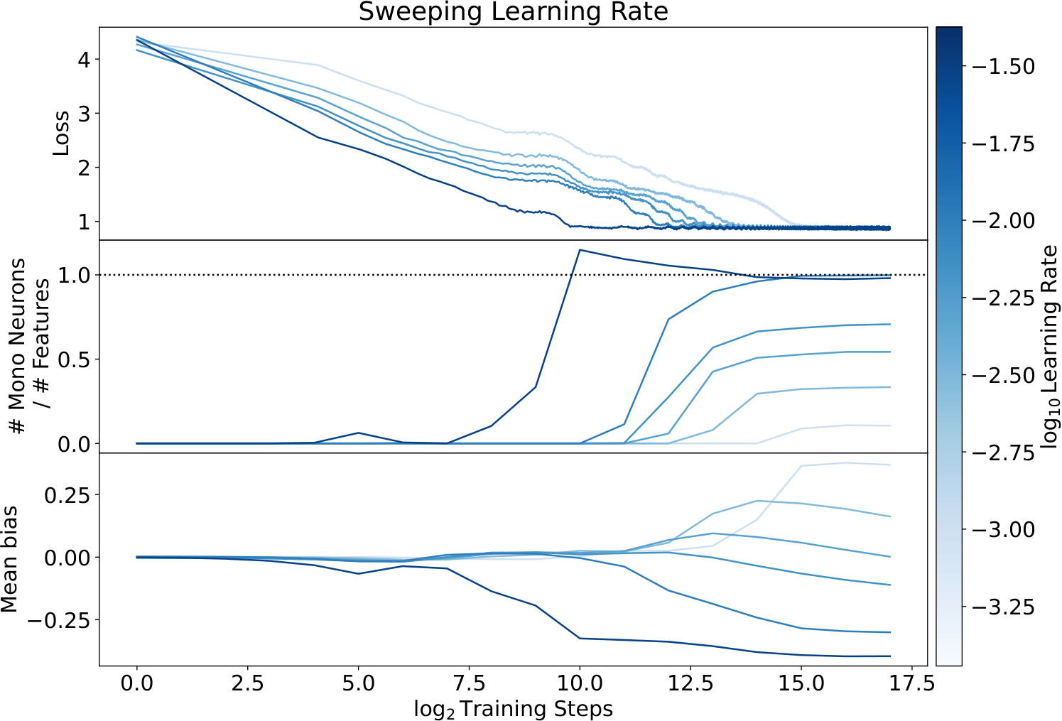
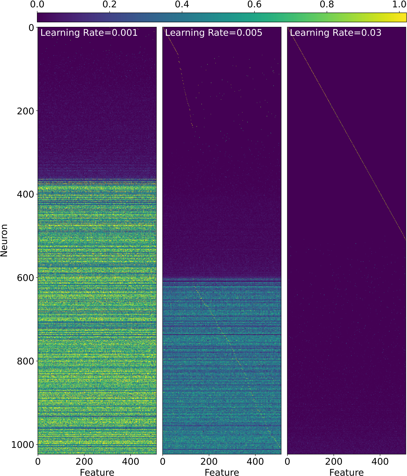
At hidden width 1,024, learning-rate changes produce markedly different neuron selectivity with nearly identical final decoder loss. Negative biases characterize selective neurons, while positive biases characterize many mixed units. Similar behavior occurs with power-law feature frequencies. Distinct basins are a plausible interpretation, not a demonstrated absence of connecting low-loss paths.
Refer to caption
Figure 3: Training traces are shown for models with different learning rates from batch LR1. Remarkably, the final models have the same loss but very different numbers of monosemantic neurons. Note that because the training samples are randomly generated anew for each batch the expected training and test losses are the same.
Refer to caption
Figure 4: The neuron activations are shown for all single-feature inputs of unit strength. Neurons are sorted by monosemanticity, with the upper-most being the most monosemantic (equation 7). Features are sorted by the neuron they activate most-strongly. The different panels show this for different final models from batch LR1 with different learning rates. These three models implement very different algorithms but achieve the same loss.
Refer to caption
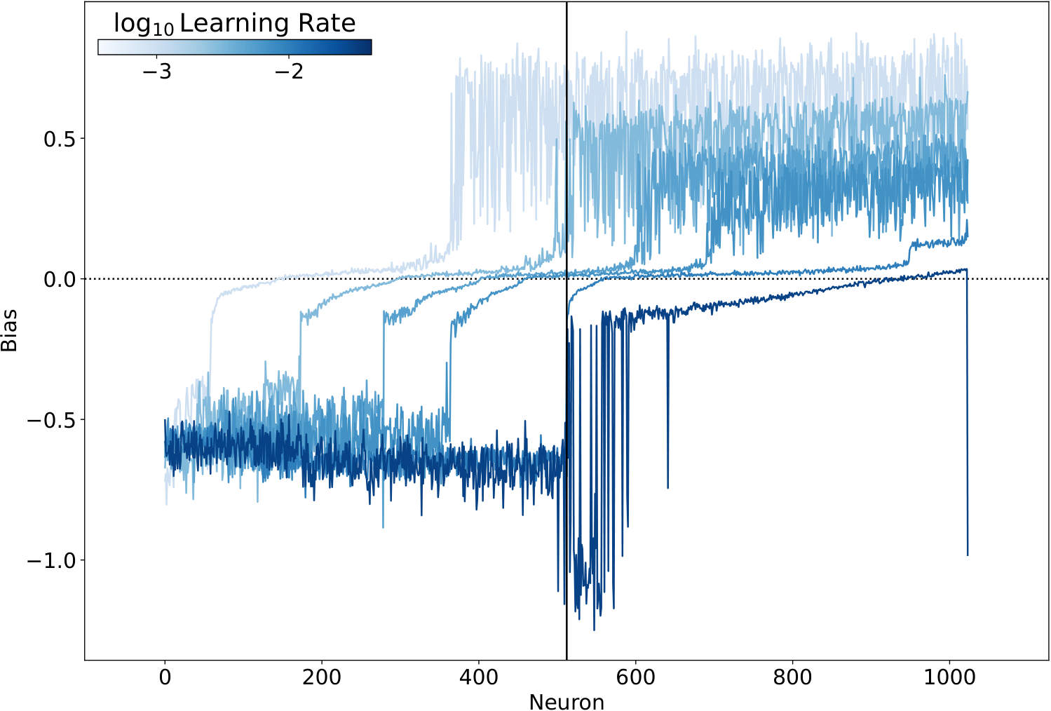
Figure 5: The neuron biases are shown for the final models from batch LR1. Neurons are sorted by monosemanticity (equation 7). Curves are colored by learning rate. The most monosemantic neurons all have moderate negative biases, while the most polysemantic have moderate positive biases.
Refer to caption
Figure 6: Training traces are shown for models with different learning rates from batch LR2. Remarkably, the final models have the same loss but very different numbers of monosemantic neurons. We also see that the number of monosemantic neurons continues to rise well after the loss plateaus. This is because there are low-frequency features which make a small difference to the loss and take a long time to learn: as these are learned, the model adds monosemantic neurons but the loss does not change much. Note that because the training samples are randomly generated anew for each batch the expected training and test losses are the same.

4.1.2 Negative Bias and Training Protocol

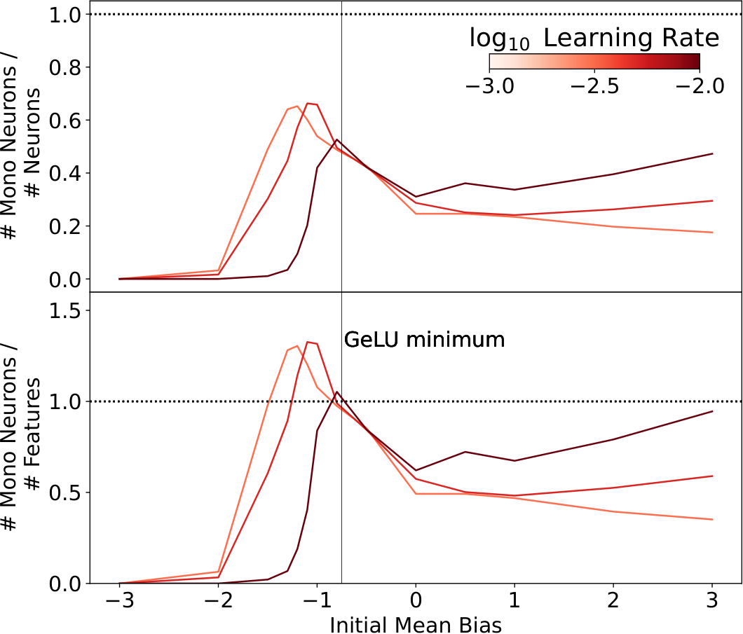
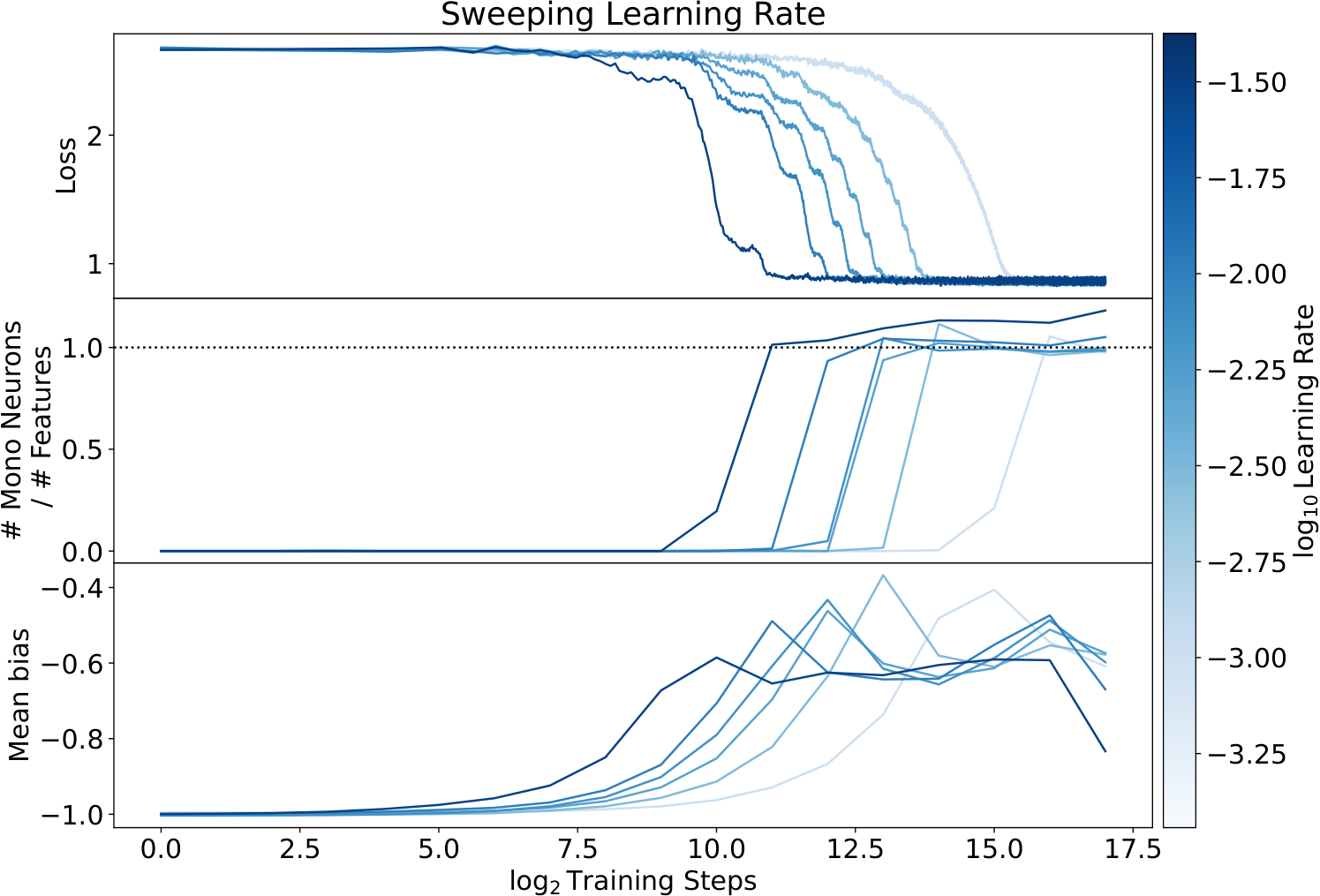
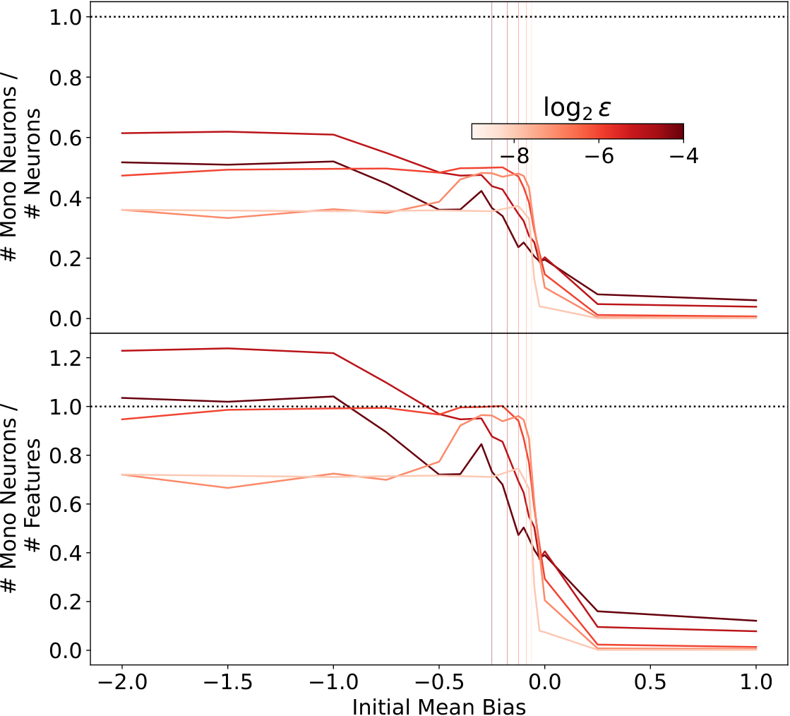
Biases start near −1 and decay until units activate; decay is disabled for the final half of training. This steers ReLU models toward selective solutions across tested learning rates. Effective starting scales depend on feature frequency, and GeLU has a preferred scale near −1. A persistent group of roughly input-dimension-many positive-bias neurons remains polysemantic.
Refer to caption
Figure 7: Training traces are shown for models with different learning rates from batch LR3. Using a negative initial mean bias and weight decay allows us to ensure that models of different learning rates all find highly-monosemantic solutions.
Refer to caption
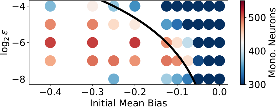
Figure 8: The fraction of neurons which are monosemantic (upper) and the ratio of monosemantic neurons to input features (lower) are shown as a function of the initial mean bias and feature density ϵ\epsilon for models from batches B1-B5. The dashed black lines show where the number of monosemantic neurons equals the number of neuronss (upper) and the number of features (lower). The vertical lines shows the scale −ϵ1/2-\epsilon^{1/2} corresponding to each curve. Both occur near where the monosemantic fraction stars dropping, indicating that the initial mean bias becomes less effective at producing monosemantic solutions once it is more positive than ≈−ϵ1/2\approx-\epsilon^{1/2}.
Refer to caption
Figure 9: The number of monosemantic neurons are shown as a function of the initial mean bias and feature density ϵ\epsilon for models from batches B1-B5. The sharp dropoff in monosemanticity corresponds roughly to crossing the bias scale −ϵ1/2-\epsilon^{1/2} (black curve), indicating that the initial mean bias becomes less effective at producing monosemantic solutions once it is more positive than ≈−ϵ1/2\approx-\epsilon^{1/2}.
Refer to caption
Figure 10: The neuron activations are shown for all single-feature inputs of unit strength for models with differen learning rates from batch LR3. Neurons are sorted by monosemanticity, with the upper-most being the most monosemantic (equation 7). Features are sorted by the neuron they activate most-strongly. The different panels show this for different final models from Figure 7 with different learning rates. Contrasting with Figure 4, we see that a negative initial bias results in highly monosemantic solutions across the board. There is still a cluster of polysemantic neurons, whose function is to produce a low-rank approximation of the identity (Section 5.2).
Refer to caption
Figure 11: The neuron biases are shown for the final models from batch LR3. Neurons are sorted by monosemanticity (equation 7). Curves are colored by learning rate. We see that the polysemantic neurons from Figure 10 correspond to positive-bias neurons, and that the monosemantic neurons correspond to those with negative biases. Remarkably, the width of the polysemantic band of neurons is uniform across models, exactly 65 neurons wide in each case, which is one more than the embedding dimension. We understand why the number of these neurons is near the embedding dimension (Section 5.2) but not why there should be one more.
Refer to caption
Figure 12: Training traces are shown for models with different learning rates with power-law feature frequencies from batch LR4. Using a negative initial mean bias and weight decay allows us to ensure that models of different learning rates all find highly-monosemantic solutions.
Refer to caption
Figure 13: The fraction of neurons which are monosemantic (upper) and the ratio of monosemantic neurons to input features (lower) are shown for models with GeLU activations from batch B3 as functions of the initial bias and learning rate. The dashed black lines show where the number of monosemantic neurons equals the number of neurons (upper) and the number of features (lower). The vertical line shows the location of the minimum of the GeLU. We see that the GeLU activation comes with a preferred bias scale of roughly −1-1 at which models learn highly monosemantic solutions.

4.1.3 Comparison with L1 Regularization

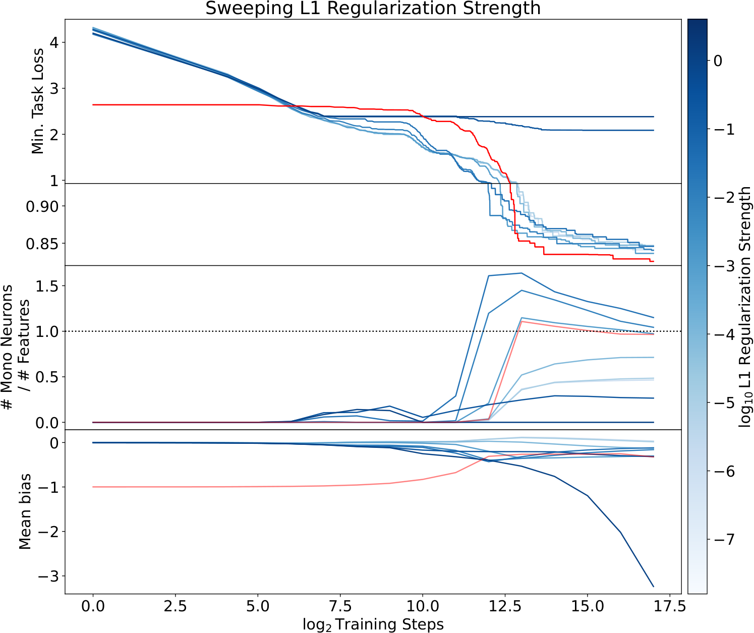
Negative-bias initialization obtains performance and selectivity comparable to the best tested L1 activation penalty. Bias decay changes the optimization path; L1 changes the objective. Both introduce task-dependent tradeoffs and may be combined rather than treated as universally competing methods.
Refer to caption
Figure 14: Training traces are shown for models with different L1 regularization strengths from batch RG1, as well as a model trained with the same parameters but no regularization and a negative initial mean bias (red). The negative initial bias model achieves lower loss and comparable monosemanticity to the best model found with L1 regularization.

4.1.4 Varying Nonlinear Dimension

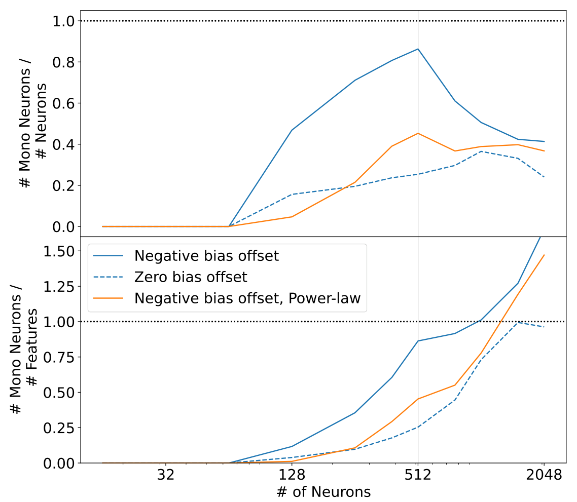
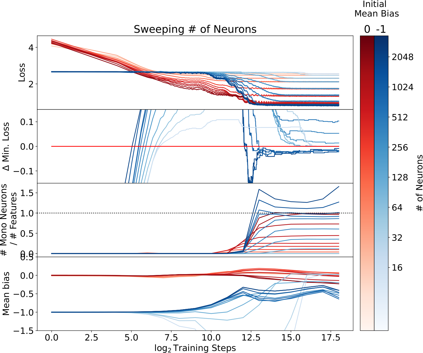
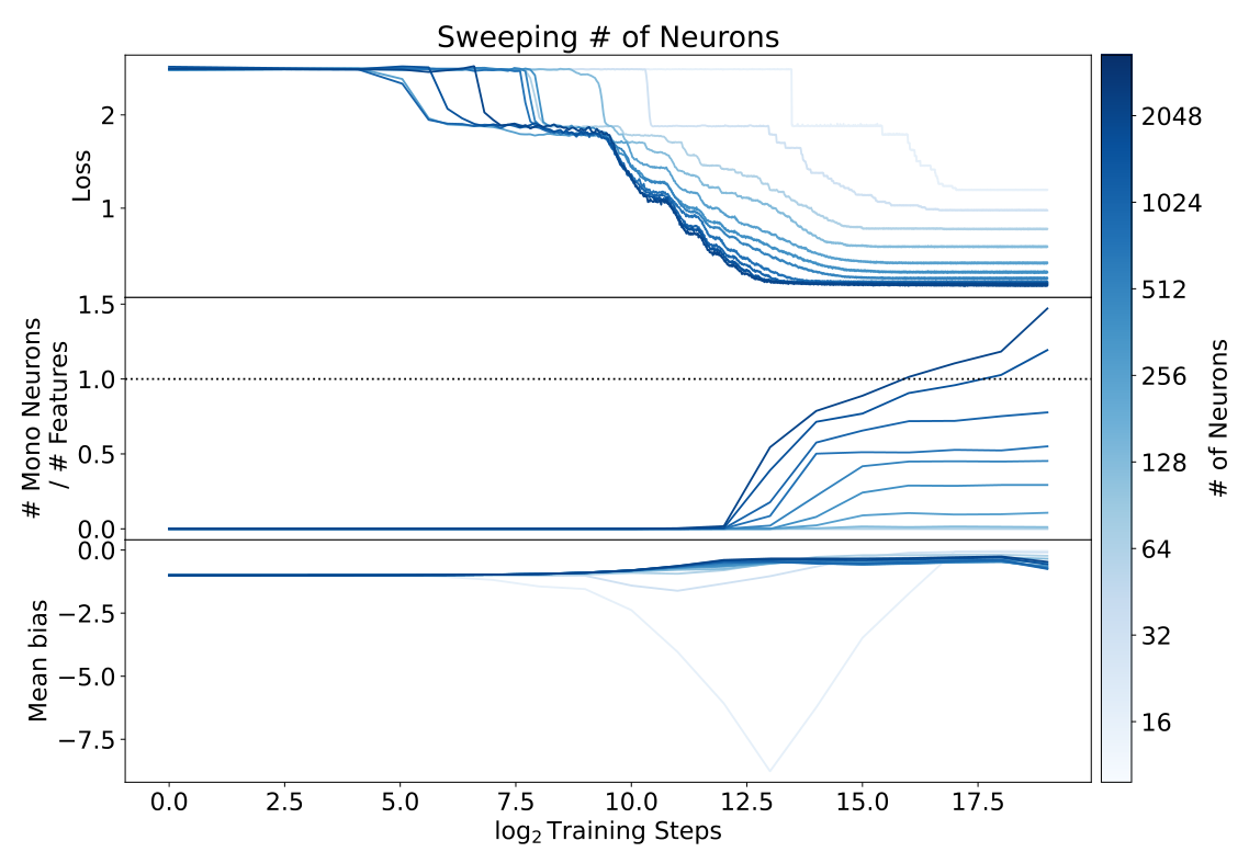
Increasing hidden width generally raises the number of selective neurons and lowers loss until width exceeds the feature count, after which loss gains diminish. At some intermediate widths the more monosemantic solution is slightly worse, while sufficiently wide models can improve both. Fixed random sparse connectivity substantially worsens loss at matched compute in the attempted efficiency experiment.
Refer to caption
Figure 15: Training traces are shown for models with different nonlinear dimensions from batch K0 with zero initial mean bias (red) and batch K1 with a negative initial mean bias (blue). Models with more neurons learn more monosemantic solutions and achieve lower loss up until the number of neurons exceeds the number of features, at which point the loss sees sharply diminishing returns with scale and additional neurons mostly just increases the number of monosemantic neurons. Models with a negative initial mean bias learn much more monosemantic representations and have very similar losses.
Figure 16: Training traces are shown for models with different nonlinear dimensions and power-law feature frequencies from batch K2. Models with more neurons learn more monosemantic solutions and achieve lower loss up until the number of neurons exceeds the number of features, at which point the loss sees sharply diminishing returns with scale and additional neurons mostly just increases the number of monosemantic neurons. Notice that the largest models continue to gain more monosemantic neurons through additional training even after the loss plateaus: we suspect that this is because the most infrequent features are still being learned and so produce more monosemantic neurons, but contribute so little to the loss that they do not make an appreciable difference there.
Figure 17: The fraction of neurons which are monosemantic (upper) and the ratio of monosemantic neurons to input features (lower) are shown for models with varying numbers of neurons from batches K0 with zero initial mean bias (blue, dashed), K1 with a negative initial mean bias (blue, solid), and K2 with a negative initial mean bias and power-law feature frequencies (orange). The dashed black lines show where the number of monosemantic neurons equals the number of neurons (upper) and the number of features (lower). The vertical line shows where the number of neurons equals the number of input features. The negative initial mean bias indeed increases monosemanticity. We also see that models have more monosemantic neurons as the total number of neurons increases, but that the fraction of neurons which are monosemantic peaks when there is one neuron per feature. We suspect that the fraction of monosemantic neurons would rise in the largest models if we allowed more training time, however, and so this trend may partially reflect the limited training time we allowed.

4.1.5 Feature Sparsity

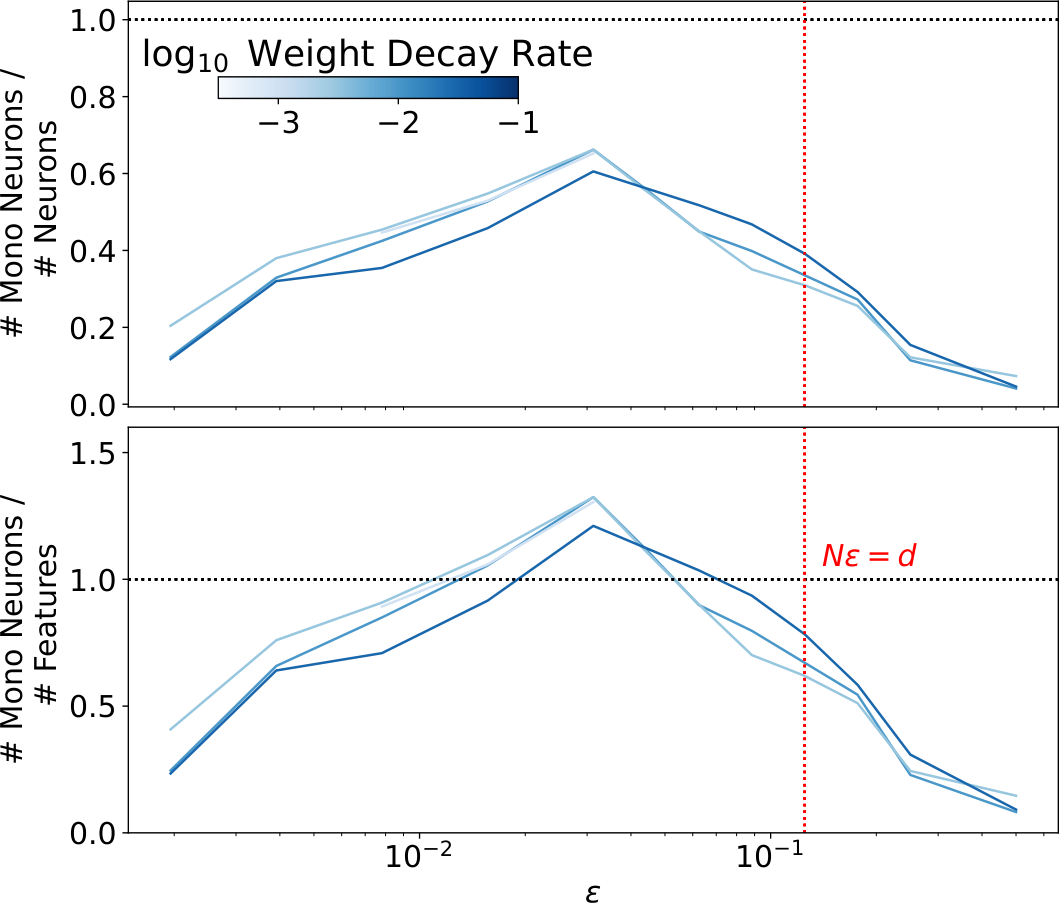
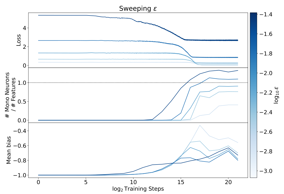
As more features co-occur, selectivity decreases smoothly around the regime where active-feature count approaches input dimension. Very rare features require slower bias decay and longer training; otherwise the bias disappears before they are learned. The observed behavior is consistent with compressed-recovery limits but does not constitute a general recovery theorem.
Refer to caption
Figure 18: The fraction of neurons which are monosemantic (upper) and the ratio of monosemantic neurons to input features (lower) are shown for models from batches E1-E4 as functions of the feature frequency ϵ\epsilon and weight decay rate. The dashed black lines show where the number of monosemantic neurons equals the number of neurons (upper) and the number of features (lower). The dashed red line shows where the expected number of features present in a sample (N​ϵN\epsilon) equals the embedding dimension dd. This line is near the transition from most features being monosemantically represented to most features being polysemantically represented. In the very sparse limit there are highly monosemantic models, but we need to use a slower weight decay and longer training runs to find them because the model sees each feature less often and so learns more slowly.
Figure 19: Training traces are shown for models with different feature sparsities from batch E3. At higher sparsity we see that the initial mean bias decays further before the loss starts to fall, resulting in models finding less monosemantic local minima.
Refer to caption
Figure 20: The neuron activations are shown for all single-feature inputs of unit strength. Neurons are sorted by monosemanticity, with the upper-most being the most monosemantic (equation 7). Features are sorted by the neuron they activate most-strongly. The different panels show this for different final models from batch E1 with different feature frequencies. No sharp phase transition is evident: rather models appear to smoothly transition from highly-monosemantic to highly-polysemantic across the boundary between the feature-sparse and feature-dense limits.

4.2 Task: Random Re-Projector

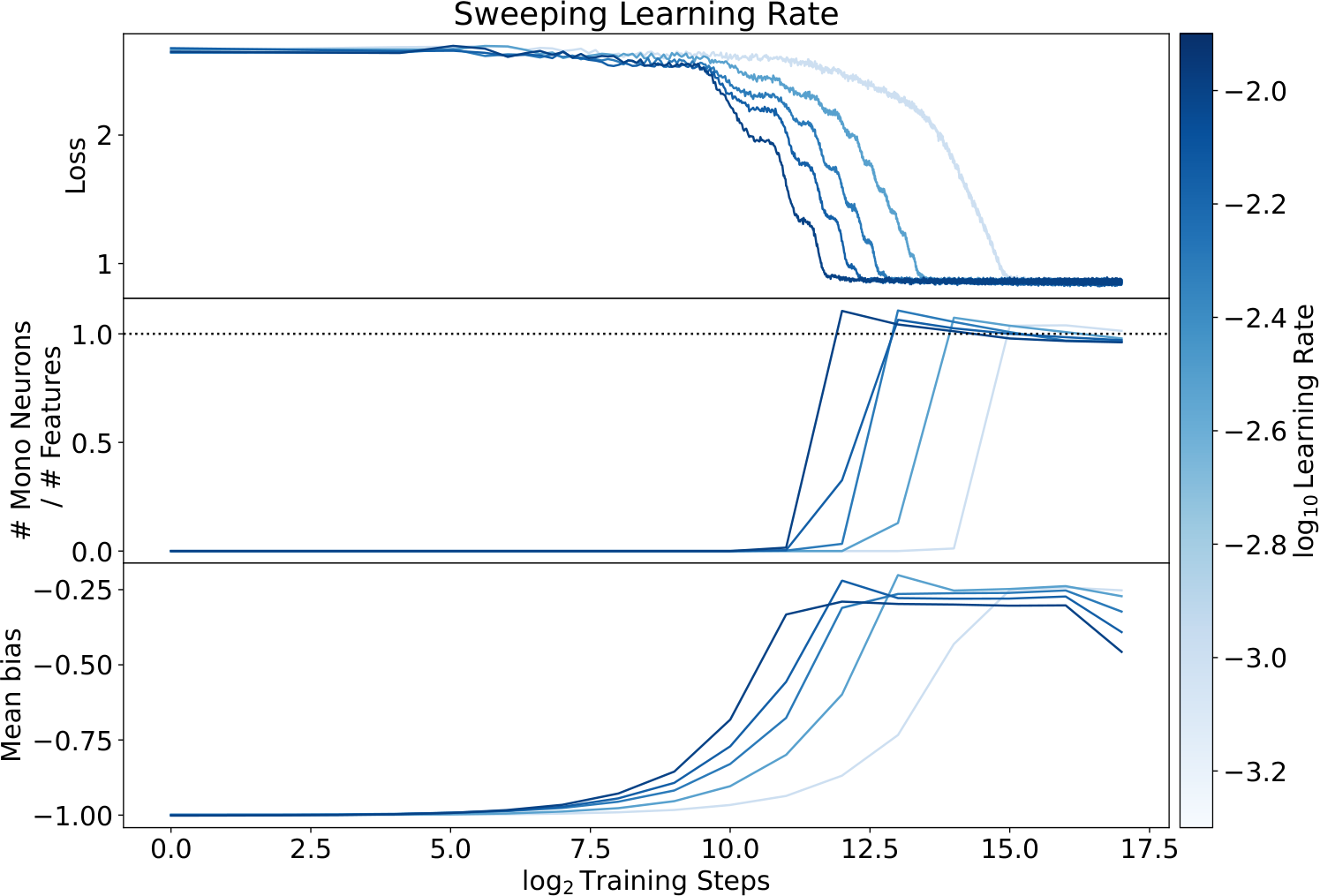
The random re-projection task also yields roughly one selective neuron per feature under negative-bias initialization across the tested learning rates. This suggests the effect is not solely a consequence of an explicitly feature-aligned output basis.
Refer to caption
Figure 21: Training traces are shown for random re-projector models with different learning rates with from batch RP1. As in the decoder models, with an initial negative bias we are able to create models with roughly one monosemantic neuron per feature across a range of learning rates.

4.3 Task: Absolute Value

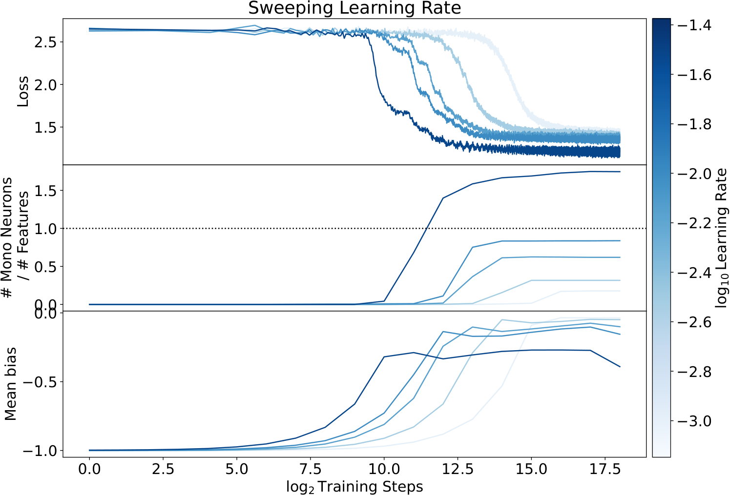
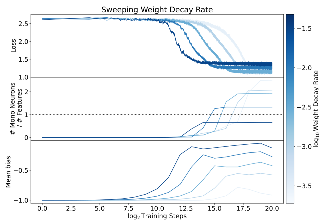
On absolute values, more monosemantic models achieve lower loss, and negative initialization alone is insufficient. Lower bias decay or a higher learning rate helps. The authors hypothesize that this harder task needs more time within a useful bias range; preliminary negative-bias regularization is left for further study.
Refer to caption
Figure 22: Training traces are shown for absolute value models with different learning rates with from batch LR5. Unlike in the decoder and re-projector models, we see that basins of different monosemanticity have different losses, with lower losses for more-monosemantic solutions. We also see here that a negative initial bias alone is not enough to ensure a highly monosemantic solution: the monosemanticity rises with increasing learning rate.
Figure 23: Training traces are shown for absolute value models with different weight decay rates with from batch D1. Slower weight decay rates produce more monosemantic solutions.

5 Mechanistic Interpretability

The mechanistic analysis focuses on highly monosemantic feature decoders, splitting units approximately into negative-bias selective and positive-bias mixed groups. It does not explain the most polysemantic models or every task.

5.1 Monosemantic Neurons

A single selective ReLU suppresses weak apparent features that may be projection interference, then estimates stronger features. Two selective neurons provide an additional bend, improving the transition to near-faithful recovery at high amplitude. Lower feature frequency shifts the thresholds downward, consistent with reduced interference rather than redundant duplicate encoding.
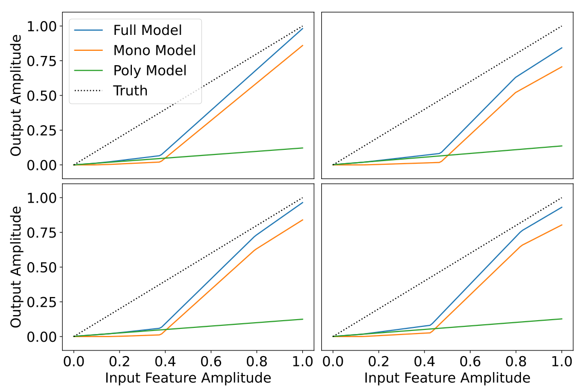
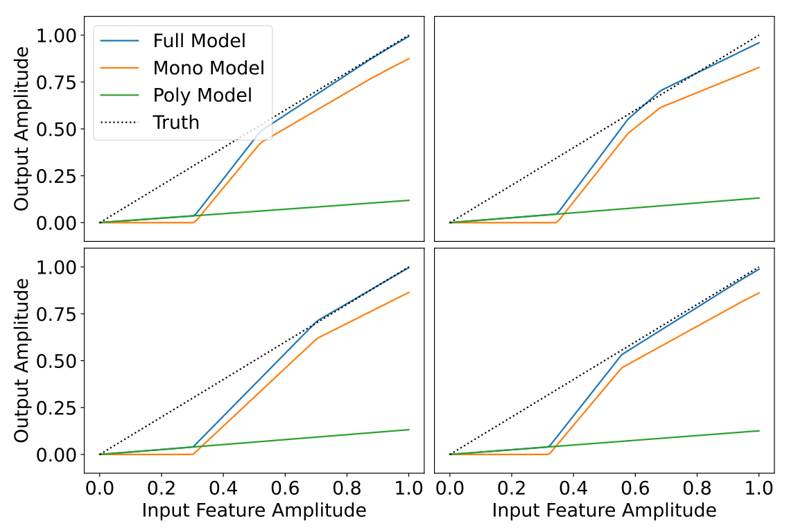
Figure 24: The outputs of a final model from batch E1 with ϵ = 1 / 64 \epsilon=1/64 are shown for four features as a function of input feature amplitude for samples containing just one active feature. The output is shown for the full model (blue), the monosemantic portion (orange), and the polysemantic portion (green). Exact recovery is marked by the dotted line. The upper left panel shows a feature primarily represented by a single monosemantic neuron, while the remaining three panels show features primarily represented by a pair of monosemantic neurons each. Note that the additional neuron is not there for redundancy, rather it allows the model to express a more fine-grained notion of confidence in the feature.
Figure 24: The outputs of a final model from batch E1 with ϵ=1/64\epsilon=1/64 are shown for four features as a function of input feature amplitude for samples containing just one active feature. The output is shown for the full model (blue), the monosemantic portion (orange), and the polysemantic portion (green). Exact recovery is marked by the dotted line. The upper left panel shows a feature primarily represented by a single monosemantic neuron, while the remaining three panels show features primarily represented by a pair of monosemantic neurons each. Note that the additional neuron is not there for redundancy, rather it allows the model to express a more fine-grained notion of confidence in the feature.
Figure 25: The outputs of a final model from batch E3 with ϵ = 1 / 256 \epsilon=1/256 are shown for two features as a function of input feature amplitude for samples containing just one active feature. The output is shown for the full model (blue), the monosemantic portion (orange), and the polysemantic portion (green). Exact recovery is marked by the dotted line. Because this model was trained with a lower feature frequency than that of Figure 24 , it is more confident that the features are not due to interference and so produces non-zero output for lower-amplitude inputs and produces outputs which are closer to the ground truth for strong-amplitude inputs.
Figure 25: The outputs of a final model from batch E3 with ϵ=1/256\epsilon=1/256 are shown for two features as a function of input feature amplitude for samples containing just one active feature. The output is shown for the full model (blue), the monosemantic portion (orange), and the polysemantic portion (green). Exact recovery is marked by the dotted line. Because this model was trained with a lower feature frequency than that of Figure 24, it is more confident that the features are not due to interference and so produces non-zero output for lower-amplitude inputs and produces outputs which are closer to the ground truth for strong-amplitude inputs.

5.2 Polysemantic Neurons

The remaining positive-bias units approximately supply a low-rank linear correction to all outputs. In the inspected model, its nonzero singular values lie around 0.99–1.03, and bias contributions nearly cancel. This helps explain why about one input-dimension’s worth of mixed units remains, though the exact excess count is unexplained.
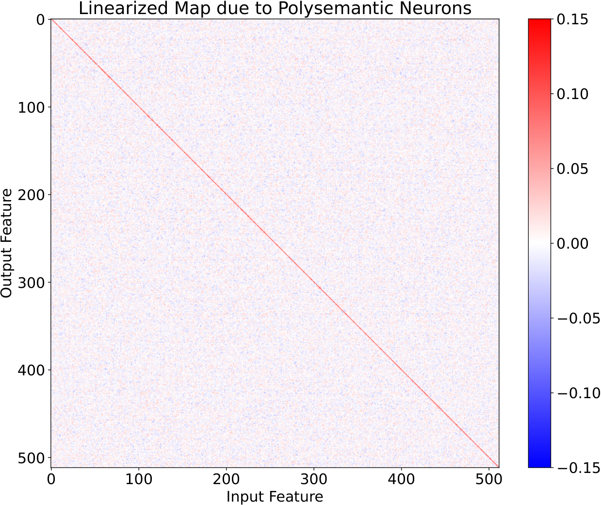
Refer to caption
Figure 26: The linearized map from input features to output features is shown for the polysemantic (positive-bias) neurons of a final model from batch E1 with ϵ=1/64\epsilon=1/64. This is close to a representation of the identity, with singular values that are all either zero or nearly-unity (0.99−1.030.99-1.03). This provides evidence that the polysemantic neurons implement a linear model with similar slopes across neurons.

5.3 Summary

The interpreted decoder combines thresholded feature-specific estimates with a shared approximately linear correction. This accounts for selected high-selectivity models; the algorithm of highly polysemantic solutions remains an open question.

6 Conclusions

The findings motivate optimization strategies that favor interpretable representations, but the current bias schedule is fragile and width costs extra computation. The equal-loss result depends on the synthetic task and available capacity. Better schedules, efficient wide layers, and interpretation of mixed solutions remain future work.

Author Contributions

Adam S. Jermyn designs and runs the experiments and leads writing. Nicholas Schiefer contributes training and bias-method ideas; Evan Hubinger contributes interpretation and activation-function analysis.

Acknowledgments

The authors acknowledge discussions, suggested tasks and comparisons, and computational support from colleagues and Hofvarpnir Studios.

Appendix A Training Details

Training uses LAMB with batch size 2²³ divided by hidden width and a cosine learning-rate schedule. The retained table specifies all run families, feature distributions, dimensions, learning rates, decay rates, and bias choices. Training examples are newly generated each batch, so expected training and test losses coincide under the same synthetic distribution.

Table 1: Training parameters and model architectures.
Batch Task Activation Feature Dist. NN mm kk ϵ\epsilon Learning Rate Decay Rate Bias Offset L1 Reg.
LR1 Decoder ReLU Uniform 512 64 1024 1/64 Variable 0 0 0
LR2 Decoder ReLU Power-law 512 64 1024 1/64 Variable 0 0 0
LR3 Decoder ReLU Uniform 512 64 1024 1/64 Variable 0.03 -1 0
B1 Decoder ReLU Uniform 512 64 1024 1/16 0.003 0.03 Variable 0
B2 Decoder ReLU Uniform 512 64 1024 1/32 0.003 0.003 Variable 0
B3 Decoder ReLU Uniform 512 64 1024 1/64 0.003 0.003 Variable 0
B4 Decoder ReLU Uniform 512 64 1024 1/128 0.003 0.003 Variable 0
B5 Decoder ReLU Uniform 512 64 1024 1/256 0.003 0.003 Variable 0
LR4 Decoder ReLU Power-law 512 64 1024 1/64 Variable 0.03 -1 0
B3 Decoder GeLU Uniform 512 64 1024 1/64 Variable 0.03 Variable 0
E1 Decoder ReLU Uniform 512 64 1024 Variable 0.003 0.03 -1 0
E2 Decoder ReLU Uniform 512 64 1024 Variable 0.003 0.01 -1 0
E3 Decoder ReLU Uniform 512 64 1024 Variable 0.003 0.003 -1 0
E4 Decoder ReLU Uniform 512 64 1024 Variable 0.003 0.001 -1 0
K0 Decoder ReLU Uniform 512 64 Variable 1/64 0.007 0 0 0
K1 Decoder ReLU Uniform 512 64 Variable 1/64 0.007 0.03 -1 0
K2 Decoder ReLU Power-law 512 64 Variable 1/64 0.007 0.03 -1 0
RG1 Decoder ReLU Uniform 512 64 1/64 0.005 0.03 -1 Variable
RP1 Re-Projector ReLU Uniform 512 64 1/64 Variable 0.03 -1 0
LR5 Abs. ReLU Uniform 512 64 2048 1/64 Variable 0.03 -1 0
D1 Abs. ReLU Uniform 512 64 2048 1/64 0.007 Variable -1 0
Concept demonstration

Open image ↗