Intuition. Imagine animating a cloud of random points into realistic data. The model learns a local arrow at each position and time, rather than simulating every complete animation during training. A point x and time t go into the network; a velocity vector comes out.
Reading the math. Training matches the predicted velocity vθ(t, x) to a constructed target ut using squared error. For an ideal straight path from noise z to data a, xt = (1−t)z + ta has velocity a−z. This conditional example explains the regression target; it does not guarantee globally shortest transport. Generation still follows the learned arrows with a differential-equation solver.
Flow Matching trains a continuous normalizing flow by regressing a neural vector field against analytically constructed conditional targets. Training samples a time, a data point, and a point on a conditional probability path, without simulating the model ODE. Conditional Flow Matching has the same expected parameter gradient as the generally intractable marginal objective. Gaussian paths include diffusion-style paths and a linear mean/scale interpolation that is optimal transport between each pair of conditional Gaussian endpoints. Image experiments favor the latter in the tested likelihood, sample-quality, and sampling-cost comparisons. Sampling and likelihood evaluation still require numerical ODE integration.
1 Introduction
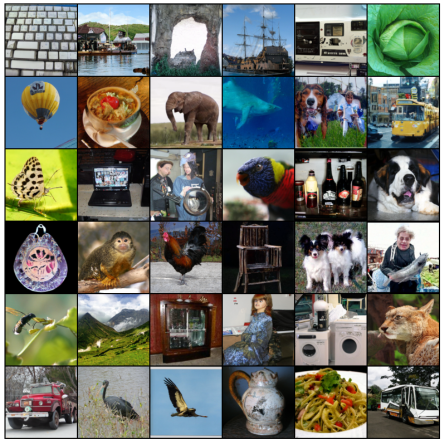
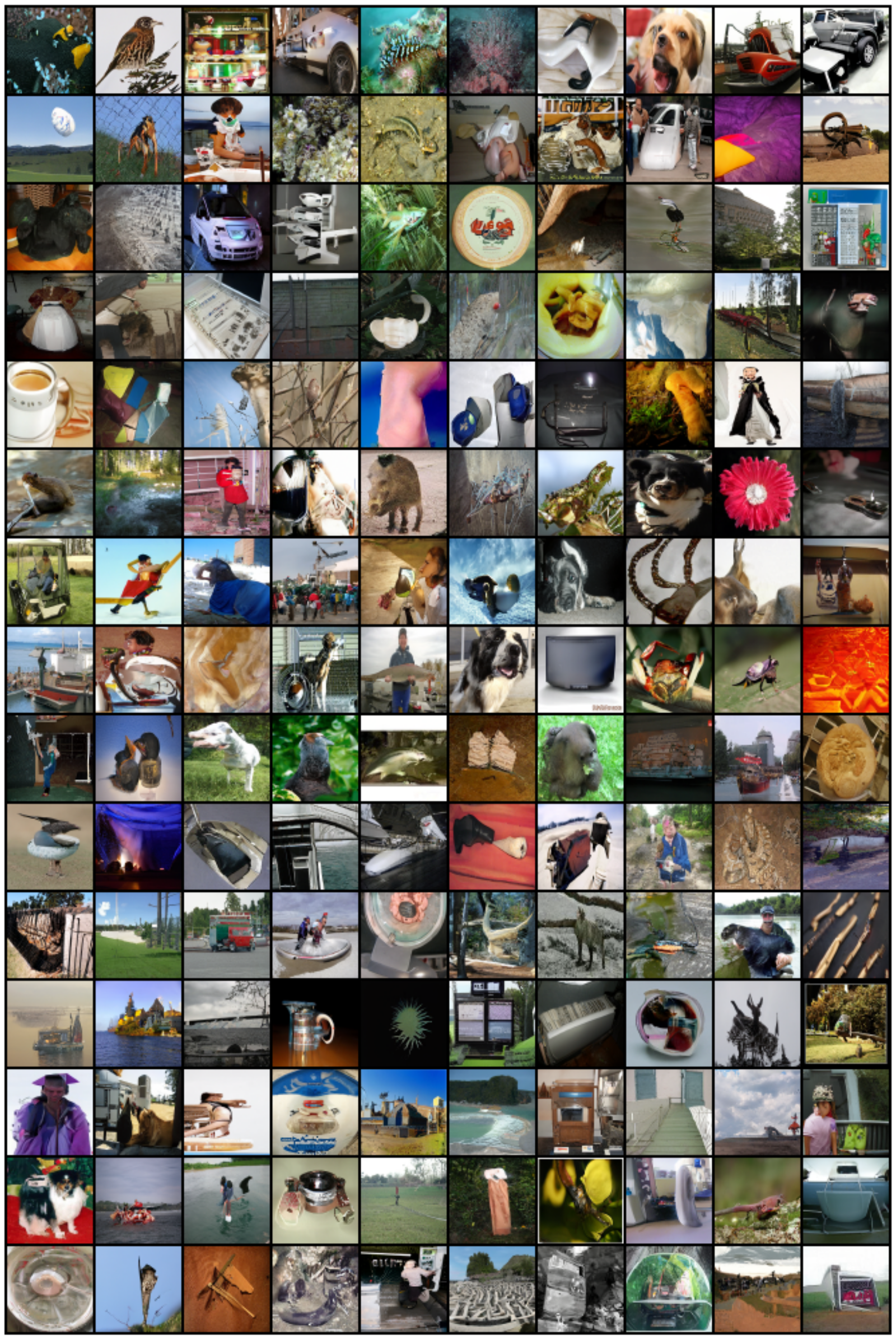
Likelihood-based training of continuous normalizing flows can require costly forward and backward ODE solves. Flow Matching instead specifies a path of distributions and learns a field that generates it. The key construction uses simple per-data-point paths and a conditional regression objective whose expected gradient matches the marginal objective. This extends simulation-free training beyond the particular paths of standard diffusion processes. The report evaluates these ideas on image generation and super-resolution; the opening sample grid is selected, while later appendix grids are labeled non-curated.
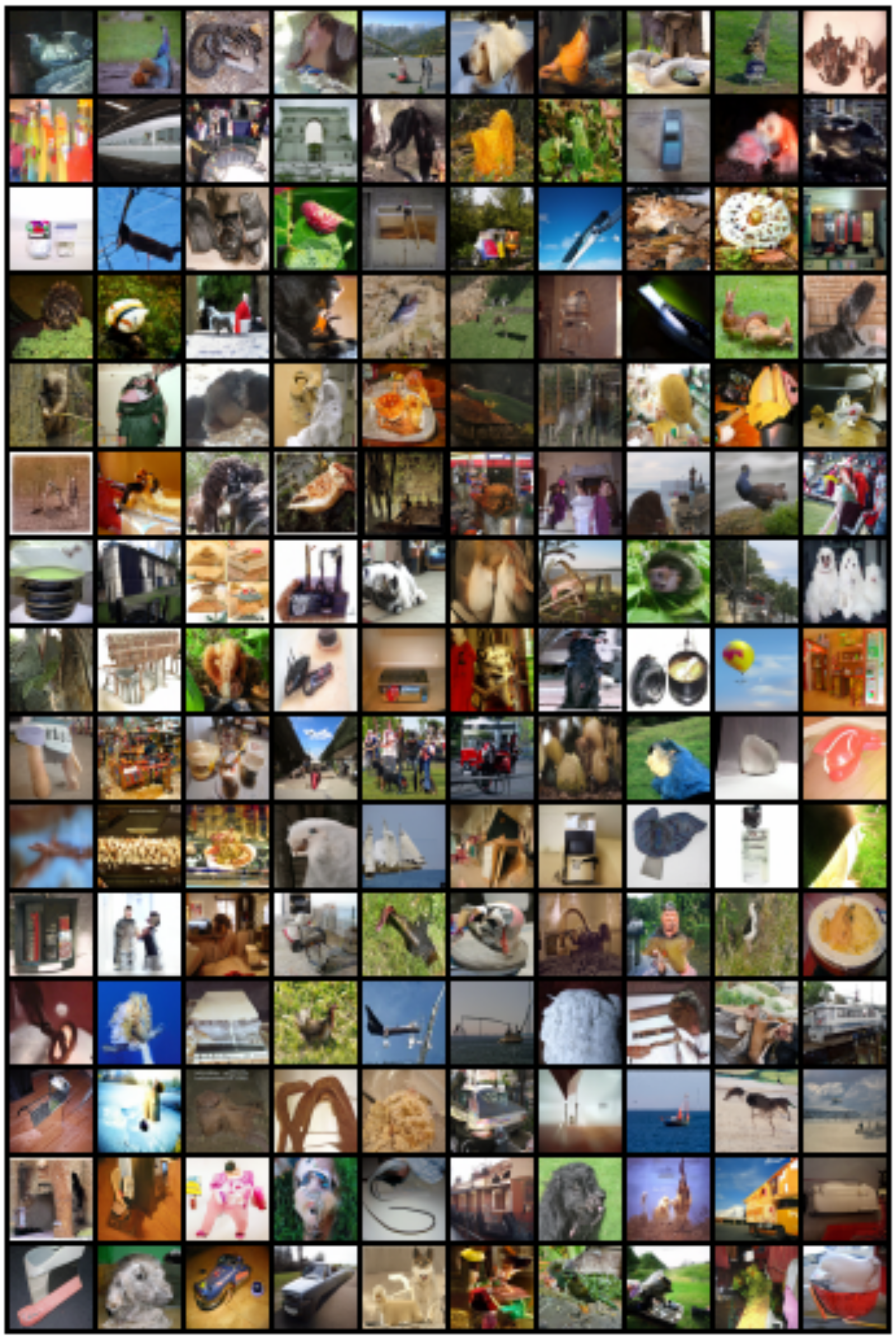
Figure 1: Unconditional ImageNet-128 samples of a CNF trained using Flow Matching with Optimal Transport probability paths.
2 Preliminaries: Continuous Normalizing Flows
A time-dependent vector field defines a flow through an ODE and transports a simple initial density into a more complex distribution. A neural parameterization gives a continuous normalizing flow. Under the required existence, uniqueness, and invertibility conditions, the change-of-variables formula defines its density; the continuity equation relates that density path to the field. These mathematical conditions matter: an arbitrary neural field is not automatically a globally well-behaved diffeomorphism. The construction follows the neural-ODE framework [Chen et al., 2018].
Equations 1–4
(1)
(2)
(3)
(4)
3 Flow Matching
The ideal objective is expected squared error between the learned field and a target field along a prescribed density path. Zero population loss would recover that field on the relevant distribution and generate the target path under the stated regularity conditions. In practice, neither the marginal density nor its field is directly available. The next sections construct them through conditional mixtures and replace the intractable regression target. The final target is a smoothed approximation to the data distribution when the endpoint noise is positive.
Equation 5
(5)
3.1 Constructing p t , u t from conditional probability paths and vector fields
For each data point x₁, a conditional path begins at a common noise distribution and ends in a narrow distribution around x₁. Averaging these densities over the data distribution defines the marginal path. The corresponding marginal field is a posterior-weighted average of conditional fields at the current position, not an unweighted average over data examples. Theorem 1 proves that this field satisfies the continuity equation for the mixture, assuming the differentiation and integration exchanges used in the proof are valid.
Equations 6–8
(6)
(7)
(8)
3.2 Conditional Flow Matching
Conditional Flow Matching samples x₁ and a point from its conditional path, then regresses the network against the conditional field. Theorem 2 shows that its expected loss differs from the marginal Flow Matching loss only by a parameter-independent constant, so their gradients and optima coincide. This does not make every stochastic gradient identical, guarantee successful optimization, or make the conditional loss vanish when the marginal field is correct; conditional targets can have irreducible variance.
Equation 9
(9)
4 Conditional Probability Paths and Vector Fields
The chosen family uses isotropic Gaussian conditional paths with time-dependent mean μₜ and positive standard deviation σₜ. An affine map ψₜ(x)=σₜx+μₜ generates each path, giving velocity (σ′ₜ/σₜ)(x−μₜ)+μ′ₜ. Reparameterization permits sampling noise x₀ directly and regressing against the time derivative of ψₜ(x₀). Theorem 3 gives the unique field for this specified invertible affine flow, not the only possible field that transports the same densities. A positive endpoint scale σ_min keeps the construction nonsingular while leaving residual smoothing.
Equations 10–15
(10)
(11)
(12)
(13)
(14)
(15)
4.1 Special instances of Gaussian conditional probability paths
Differentiable mean and scale schedules satisfying the endpoint conditions yield many possible Gaussian paths. The paper compares diffusion-derived schedules with linear interpolation between conditional Gaussian endpoints.
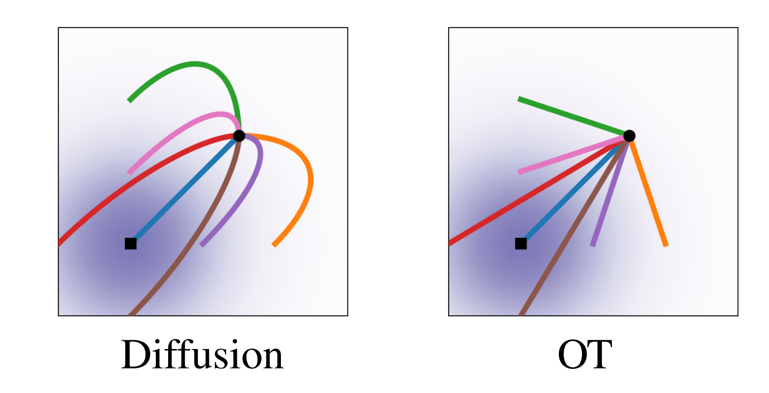
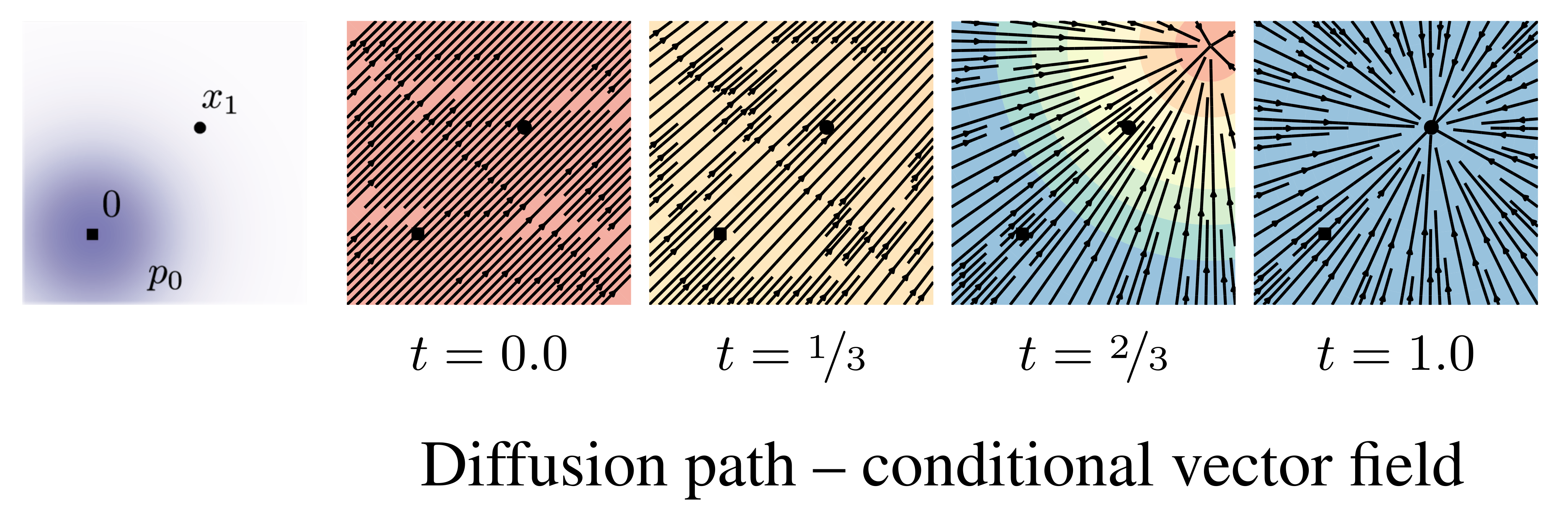
Variance-exploding and variance-preserving diffusion paths recover familiar probability-flow vector fields after reversing time to run from noise to data. The derivations preserve the required square roots, time reversals, and signs. Standard finite-time diffusion schedules only approximate a pure noise endpoint, whereas the proposed path design can impose its endpoint directly. Figure 2 contrasts a diffusion conditional score with an OT conditional vector field, so it compares different regression targets rather than claiming the two pictures show the same quantity. The connection to probability-flow ODEs is grounded in the diffusion formulation [Song et al., 2020b].
Equations 16–19
(16)
(17)
(18)
(19)
Figure 2: Compared to the diffusion path’s conditional score function, the OT path’s conditional vector field has constant direction in time and is arguably simpler to fit with a parametric model. Note the blue color denotes larger magnitude while red color denotes smaller magnitude.
The proposed mean is tx₁ and the scale is 1−(1−σ_min)t. A noise point follows a straight conditional trajectory with constant velocity x₁−(1−σ_min)x₀, yielding a particularly simple regression target. This is the Wasserstein-2 displacement interpolation between the standard Gaussian and the narrow Gaussian centered on a particular data point [McCann, 1997]. The paper explicitly warns that averaging these conditional constructions does not make the marginal field an optimal-transport solution. Consequently, straight conditional paths do not prove that every trajectory of the learned marginal flow is straight.
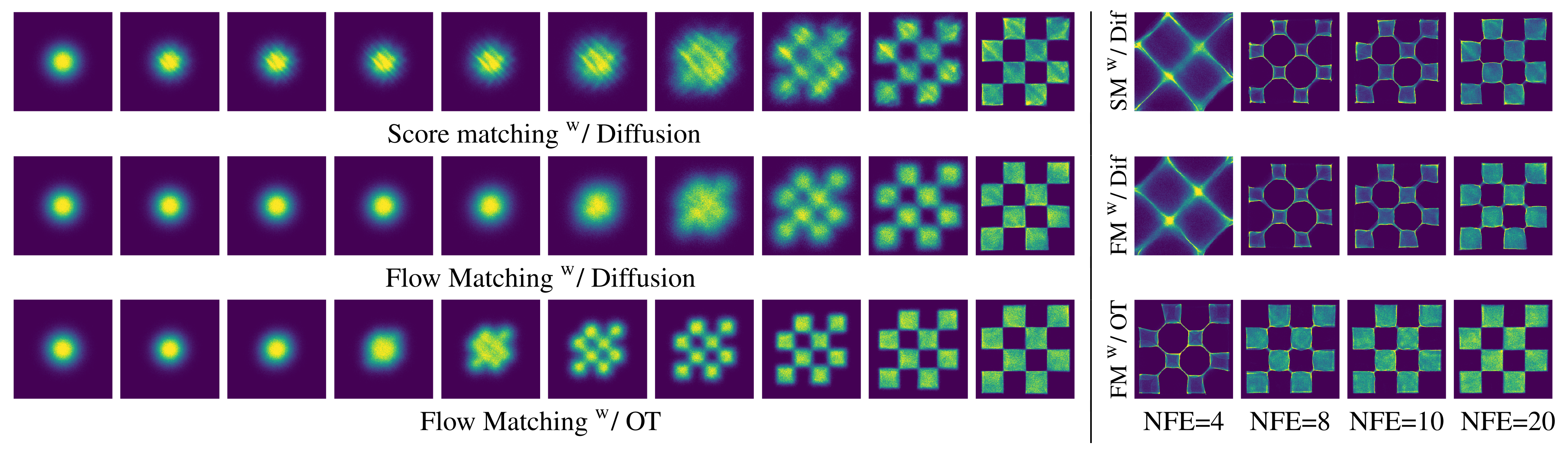
Earlier CNFs use likelihood-based ODE training or regularization to simplify integration. Other simulation-free approaches face difficult integrals or biased mini-batch gradients in the cited formulations. Conditional Flow Matching takes inspiration from denoising score matching while regressing vector fields directly and permitting more general paths. The paper also acknowledges finite-time diffusion-bridge approaches and concurrent conditional-objective work. The checkerboard experiments illustrate differences in learned density evolution and low-step integration; they are qualitative evidence for this setting rather than a general ranking of all flow or diffusion methods.
Figure 4: (left) Trajectories of CNFs trained with different objectives on 2D checkerboard data.
The OT path introduces the checkerboard pattern much earlier, while FM results in more stable training.
(right) FM with OT results in more efficient sampling, solved using the midpoint scheme.
6 Experiments
Experiments use CIFAR-10 and ImageNet at 32, 64, and 128 pixels, plus conditional super-resolution. Unless specified otherwise, evaluation uses the adaptive Dormand–Prince solver with absolute and relative tolerances 10⁻⁵. Table 1 preserves likelihood in bits per dimension, FID, and function-evaluation counts separately. Lower values favor the model for all three metrics, but they assess different properties.
Table 1: Likelihood (BPD), quality of generated samples (FID), and evaluation time (NFE) for the same model trained with different methods.
6.1 Density Modeling and Sample Quality on ImageNet
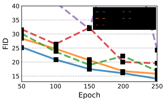
The ablations use a shared U-Net-style architecture and broadly matched training settings, with some baselines allowed extra iterations for convergence. FM with the OT path has the best reported likelihood, FID, and mean function-evaluation count across the three matched dataset columns. For ImageNet-64 it reports 3.31 BPD, FID 14.45, and 138 evaluations. CIFAR-10FIDs are worse than commonly reported values elsewhere, which the authors attribute to an architecture not tuned for that dataset. The ImageNet-128 FID of 20.9 is compared with the selected unconditional baselines; a self-supervised conditioned model is excluded. Training-throughput comparisons also change batch size and model size, including a 25% larger FM model, so fewer iterations alone are not a matched-compute speedup.
Figure 5: Image quality during training, ImageNet 6464.
6.2 Sampling Efficiency
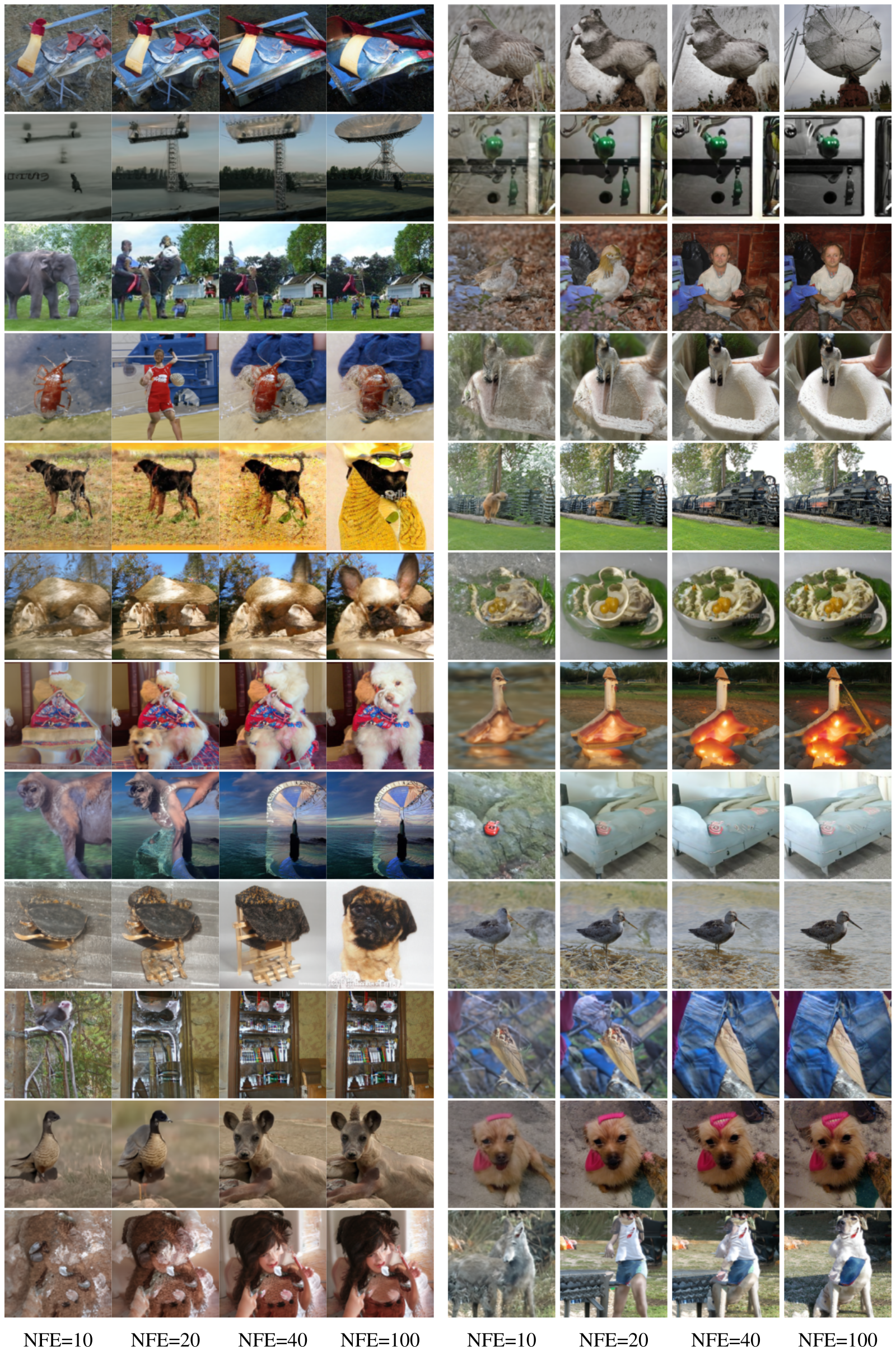
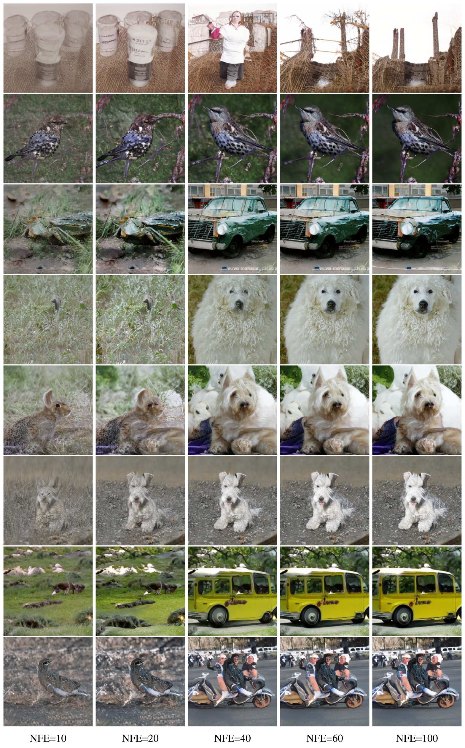
Sampling starts from Gaussian noise and integrates the learned vector field. Image sequences and checkerboard examples show earlier emergence of structure under the OT-path recipe. Fixed-step tests compare numerical error with a 1,000-evaluation reference using 256 seeds; FM-OT needs roughly 60% as many evaluations to reach the illustrated error level. FID-versus-evaluation curves favor it among the tested objectives and solvers. These are empirical numerical and perceptual trade-offs, not guarantees for every solver, tolerance, image, or learned field. The appendix retains same-seed examples at multiple evaluation counts.
Figure 6: Sample paths from the same initial noise with models trained on ImageNet 6464. The OT path reduces noise roughly linearly, while diffusion paths visibly remove noise only towards the end of the path. Note also the differences between the generated images.Figure 7: Flow Matching, especially when using OT paths, allows us to use fewer evaluations for sampling while retaining similar numerical error (left) and sample quality (right). Results are shown for models trained on ImageNet 3232, and numerical errors are for the midpoint scheme.
6.3 Conditional sampling from low-resolution images
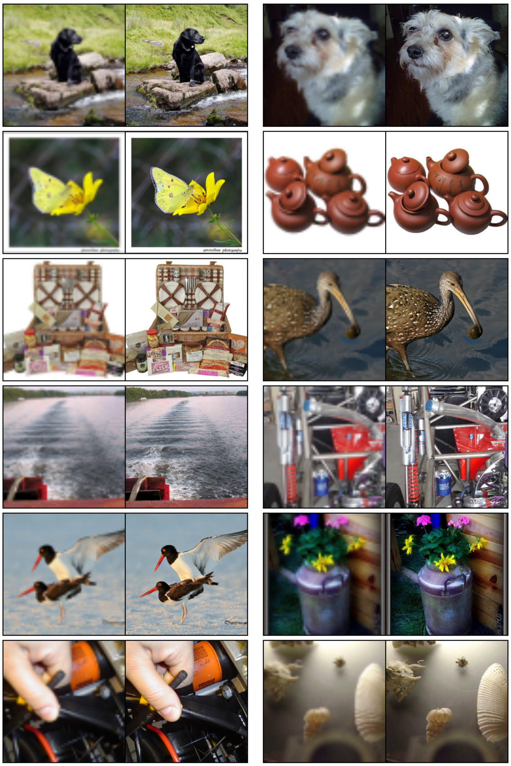
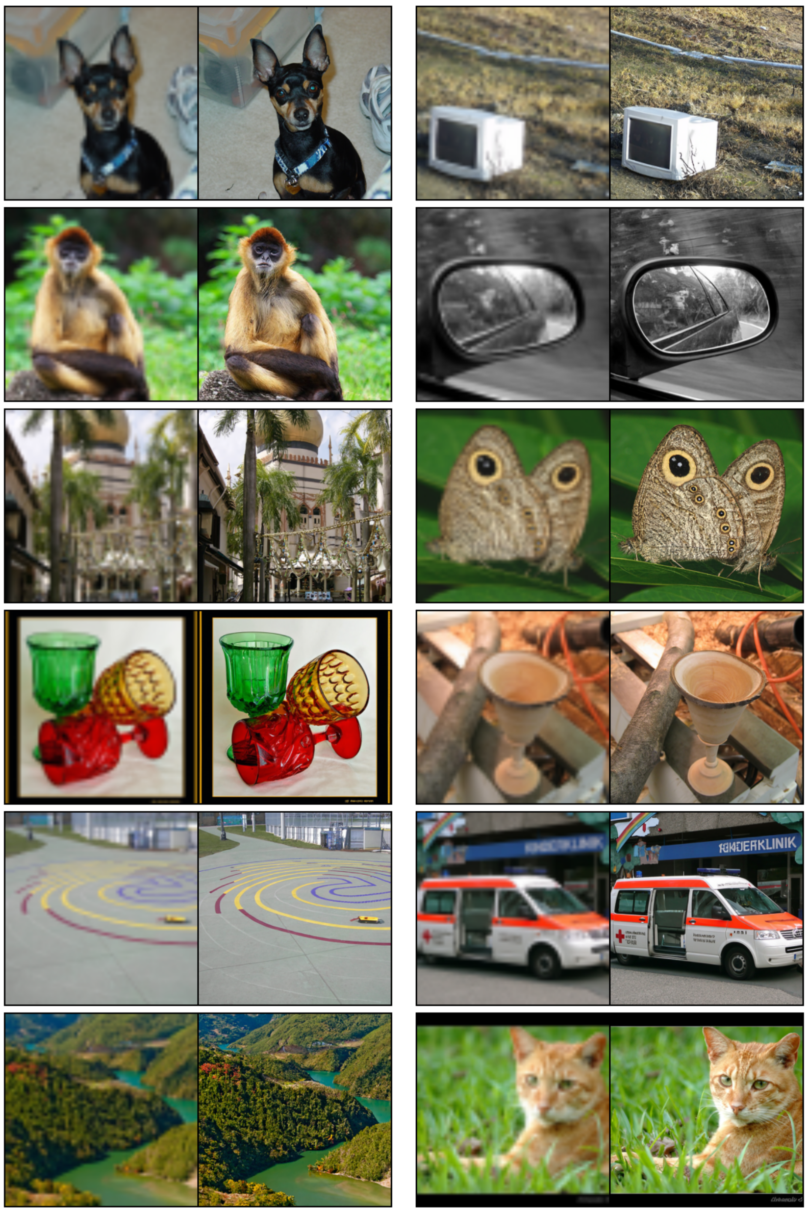
A conditional model upsamples ImageNet validation images from 64×64 to 256×256. Compared with SR3, FM-OT improves FID from 5.2 to 3.4 and Inception Score from 180.1 to 200.8, while PSNR falls from 26.4 to 24.7 and SSIM from 0.762 to 0.747. Thus distributional sample-quality metrics improve while paired-image fidelity metrics worsen; describing the result requires that trade-off. All example pairs and their low-resolution insets are preserved.
Table 2: Image super-resolution on the ImageNet validation set.
7 Conclusion
Conditional vector-field regression provides scalable training without trajectory simulation and allows paths beyond conventional diffusion schedules. The strongest empirical results here use the conditional Gaussian OT construction. More general kernels and non-isotropic paths are suggested as future work. Sampling cost, approximation error, endpoint smoothing, and the limited scope of the image benchmarks remain relevant when extending the result.
8 Social responsibility
The authors acknowledge harmful uses of generated images and suggest controlled training content and image validation as mitigations. They also motivate more efficient training as a possible way to reduce time and energy use. The paper does not provide a complete misuse-prevention method or a lifecycle energy measurement.
Appendix A Theorem Proofs
Theorem 1 averages the conditional continuity equations and exchanges integration with time differentiation and divergence under Leibniz-rule regularity. Theorem 2 expands both squared losses: the network-norm and network/target cross terms agree under the mixture identity, and the remaining target-only term is independent of the parameters. The proof assumes sufficient decay, integrability, and boundedness to justify Fubini and differentiation. Theorem 3 differentiates the affine conditional flow and substitutes its inverse, requiring σₜ>0. These proofs establish the identities under their assumptions; they do not remove finite-model, finite-data, optimization, or numerical-solver error.
Equations 25
(25)
Appendix B The continuity equation
The continuity equation ∂ₜp+div(pv)=0 expresses conservation of probability mass. Together with a suitable initial density and regular flow conditions, it connects a vector field to the density path it generates. The spatial divergence and its coordinate definition are preserved.
Equation 26
(26)
Appendix C Computing probabilities of the CNF model
The appendix explains likelihood evaluation by reverse integration, an efficient stochastic divergence estimator, correction for data transformations, and conversion to bits per dimension. Likelihood evaluation remains an ODE computation even though training is simulation-free.
Along a trajectory, the log-density derivative is minus the field divergence. To evaluate a given final point, integrate the state backward while accumulating the divergence, then combine the recovered prior log density with that accumulator. The sign and initial conditions in Equations 27–33 are retained. One preceding unnumbered HTML equation contains an unmatched-delimiter conversion marker; its visible display is restored from the exact PDF, with original MathML retained in a disclosure.
Equations 27–33
Original source MathML (contains a conversion marker for an unmatched delimiter)
(27)
(28)
(29)
(30)
(31)
(32)
(33)
Unbiased estimator to p 1 ( x 1 )
Hutchinson’s estimator replaces a full Jacobian trace by zᵀDv z with E[zzᵀ]=I. Along the exact deterministic state trajectory and under the stated integrability assumptions, the resulting accumulated quantity is an unbiased estimator of log p₁. Although this subsection’s heading and final sentence refer to p₁, its proof and Equation 35 establish log-density unbiasedness. Exponentiating that estimator is generally biased, and numerical integration adds controlled approximation error. The original derivation is preserved without silently changing its claim.
Equations 34–35
(34)
(35)
Transformed data
Data centering and scaling require the corresponding change-of-variables determinant. Mapping model-space pixels from [−1,1] to [0,256] subtracts 7d log 2 from the continuous log density in the pixel coordinates. This correction is distinct from uniform dequantization of discrete pixel values.
Bits per dimension is the negative base-two log density divided by the number of scalar image coordinates. Under the stated pixel transform, the model-space expression receives an additive seven. Averaging the stochastic log-density estimator approximates the test-set BPD subject to trace-estimator variance and numerical error.
Equations 37
(37)
Appendix D Diffusion conditional vector fields
The appendix derives conditional vector fields corresponding to diffusion probability paths. Reversing a path from data-to-noise into noise-to-data negates the time-reversed vector field; the proof checks this with the continuity equation.
Equation
Conditional VFs for Fokker-Planck probability paths
For an SDE with time-dependent scalar diffusion coefficient, the Fokker–Planck equation can be rewritten as a continuity equation with field fₜ−(gₜ²/2)∇log pₜ. This deterministic probability-flow ODE shares the SDE’s one-time density marginals, not its stochastic sample trajectories. The restriction on the diffusion form matters when generalizing the formula.
The variance-exploding Gaussian conditional path yields a radial field proportional to σ′ₜ/σₜ. Time reversal produces the negative time-reversed coefficient used in the main text. Endpoint limits and finite-time noise approximations remain part of the diffusion construction.
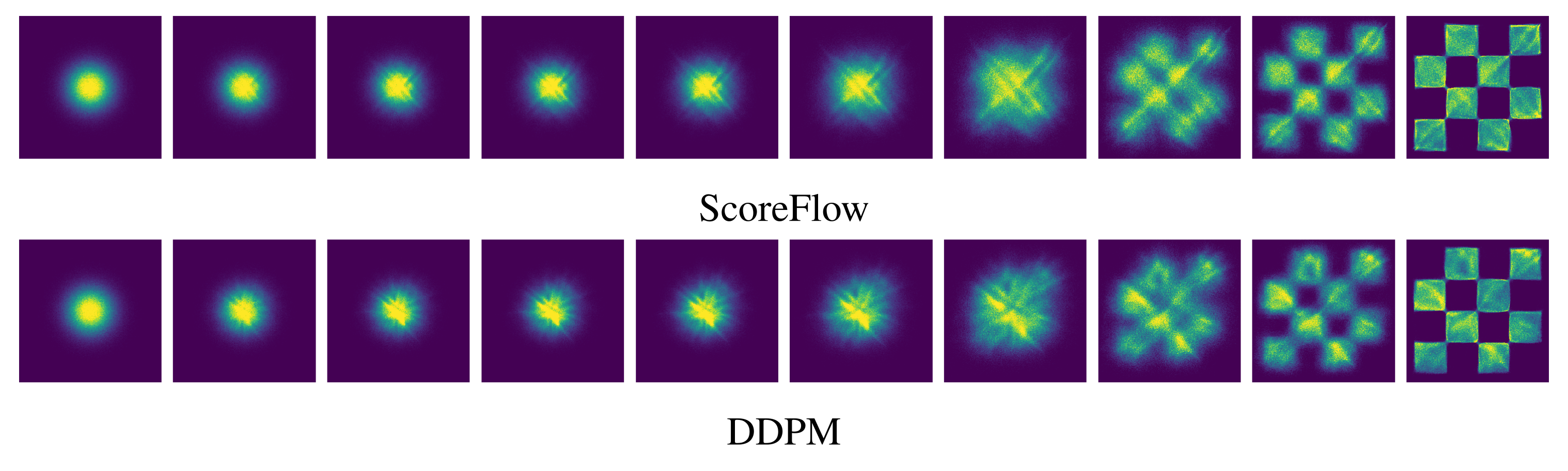
For the variance-preserving SDE, the integrated noise rate T determines both the decaying mean and variance. Substitution into the probability-flow formula and time reversal recover Equation 19. Figures 8–9 retain the conditional vector field and the additional ScoreFlow/DDPM checkerboard comparisons.
Equations 41
(41)
Figure 8: VP Diffusion path’s conditional vector field. Compare to Figure 2. Figure 9: Trajectories of CNFs trained with ScoreFlow (Song et al., 2021) and DDPM (Ho et al., 2020) losses on 2D checkerboard data, using the same learning rate and other hyperparameters as Figure 4.
Appendix E Implementation details
The two-dimensional experiments use a five-layer MLP with 512 neurons per layer. Image experiments use a U-Net architecture with the preprocessing and resolution-specific choices described in this appendix; the matched objective comparisons share the specified architecture and hyperparameters.
E.1 Diffusion baselines
Losses.
The appendix lists score-matching, likelihood-weighted ScoreFlow, and DDPM noise-prediction losses. A source sign-convention inconsistency needs care: Equation 42 describes s as the true Gaussian score, which is −(x−μ)/σ², whereas Equation 43 uses the positive residual (x−μ)/σ² as its target. The later sampling formula and noise conversion use that negative-score convention consistently. The displayed formulas remain unchanged; this notation issue alone does not establish an implementation error.
Equations 42–45
(42)
(43)
(44)
(45)
Diffusion path.
The VP schedule uses β_min=0.1 and β_max=20 with a linearly increasing noise rate. Time is truncated at 1−10⁻⁵ for the stated training, likelihood, and sampling setup to avoid the singular endpoint. All schedule formulas and their square roots are retained.
Equations
Sampling.
Sampling uses the reverse-time probability-flow expression in Equation 46. DDPM output is divided by σₜ to obtain the positive residual convention used there. This should be read alongside the score-sign qualification above, not as a definition of the conventional positive log-density gradient.
Equation 46
(46)
E.2 Training & evaluation details
Table 3 preserves all architecture, batch, GPU, epoch, iteration, and learning-rate settings. Adam uses β₁=0.9, β₂=0.999, zero weight decay, and ε=10⁻⁸. Smaller resolutions use full 32-bit training and larger ones mixed precision. Likelihood estimates use uniform dequantization and log-mean density over K samples, with adaptive integration at 10⁻⁵ tolerances. Increasing K changes the reported estimate; this nonlinear averaging is separate from the unbiased log-density trace estimator. FID implementations differ for ImageNet-128 to match the cited evaluation protocol.
Table 3: Hyper-parameters used for training each model
Equation 47
(47)
Appendix F Additional tables and figures
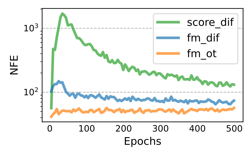
Table 4 reports dequantized BPD for several K values, while Figure 10 tracks sampling evaluations during training. Two ImageNet-32 entries differ slightly from main Table 1: the appendix gives 3.57 for score matching and 3.56 for FM with diffusion at its largest K, versus 3.56 and 3.54 in the main table. Both source tables are retained. Figures 11–13 contain all non-curated image grids; Figures 14–15 retain all super-resolution pairs. The final two same-noise, varying-NFE grids are numbered 16 and 17 in the exact v2 PDF but 17 and 18 in the generated HTML; visible captions follow the PDF while stable HTML anchors are retained. No sample panels are removed.
Table 4: Negative log-likelihood (in bits per dimension) on the test set with different values of using uniform dequantization.
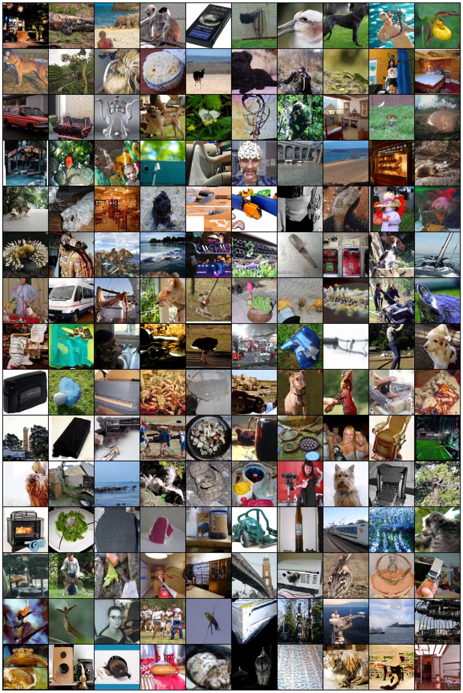
Figure 10: Function evaluations for sampling during training, for models trained on CIFAR-10 using dopri5 solver with tolerance .Figure 11: Non-curated unconditional ImageNet-32 generated images of a CNF trained with FM-OT. Figure 12: Non-curated unconditional ImageNet-64 generated images of a CNF trained with FM-OT. Figure 13: Non-curated unconditional ImageNet-128 generated images of a CNF trained with FM-OT. Figure 14: Conditional generation 6464256256. Flow Matching OT upsampled images from validation set.Figure 15: Conditional generation 6464256256. Flow Matching OT upsampled images from validation set.Figure 16:Generated samples from the same initial noise, but with varying number of function evaluations (NFE).
Flow matching with OT path trained on ImageNet-128.Figure 17:Generated samples from the same initial noise, but with varying number of function evaluations (NFE). Flow matching with OT path trained on ImageNet 256256.
52 references
Albergo & Vanden-Eijnden (2022)
Michael S Albergo and Eric Vanden-Eijnden.
Building normalizing flows with stochastic interpolants.
arXiv preprint arXiv:2209.15571, 2022.
Amodei et al. (2018)
Dario Amodei, Danny Hernandez, Girish SastryJack, Jack Clark, Greg Brockman,
and Ilya Sutskever.
Ai and compute.
https://openai.com/blog/ai-and-compute/, 2018.
Armandpour et al. (2021)
Mohammadreza Armandpour, Ali Sadeghian, Chunyuan Li, and Mingyuan Zhou.
Partition-guided gans.
In Proceedings of the IEEE/CVF Conference on Computer Vision
and Pattern Recognition, pp. 5099–5109, 2021.
Ben-Hamu et al. (2022)
Heli Ben-Hamu, Samuel Cohen, Joey Bose, Brandon Amos, Aditya Grover, Maximilian
Nickel, Ricky T. Q. Chen, and Yaron Lipman.
Matching normalizing flows and probability paths on manifolds.
arXiv preprint arXiv:2207.04711, 2022.
Casanova et al. (2021)
Arantxa Casanova, Marlene Careil, Jakob Verbeek, Michal Drozdzal, and Adriana
Romero Soriano.
Instance-conditioned gan.
Advances in Neural Information Processing Systems,
34:27517–27529, 2021.
Chen et al. (2018)
Ricky T. Q. Chen, Yulia Rubanova, Jesse Bettencourt, and David K Duvenaud.
Neural ordinary differential equations.
Advances in neural information processing systems, 31, 2018.
Chrabaszcz et al. (2017)
Patryk Chrabaszcz, Ilya Loshchilov, and Frank Hutter.
A downsampled variant of imagenet as an alternative to the cifar
datasets.
arXiv preprint arXiv:1707.08819, 2017.
De Bortoli et al. (2021)
Valentin De Bortoli, James Thornton, Jeremy Heng, and Arnaud Doucet.
Diffusion schrödinger bridge with applications to score-based
generative modeling.
(arXiv:2106.01357), Dec 2021.
doi: 10.48550/arXiv.2106.01357.
URLhttp://arxiv.org/abs/2106.01357.
arXiv:2106.01357 [cs, math, stat].
Deng et al. (2009)
Jia Deng, Wei Dong, Richard Socher, Li-Jia Li, Kai Li, and Li Fei-Fei.
Imagenet: A large-scale hierarchical image database.
In 2009 IEEE Conference on Computer Vision and Pattern
Recognition, pp. 248–255, 2009.
doi: 10.1109/CVPR.2009.5206848.
Dhariwal & Nichol (2021)
Prafulla Dhariwal and Alexander Quinn Nichol.
Diffusion models beat GANs on image synthesis.
In A. Beygelzimer, Y. Dauphin, P. Liang, and J. Wortman Vaughan
(eds.), Advances in Neural Information Processing Systems, 2021.
URLhttps://openreview.net/forum?id=AAWuCvzaVt.
Dormand & Prince (1980)
John R Dormand and Peter J Prince.
A family of embedded runge-kutta formulae.
Journal of computational and applied mathematics, 6(1):19–26, 1980.
Du et al. (2022)
Shian Du, Yihong Luo, Wei Chen, Jian Xu, and Delu Zeng.
To-flow: Efficient continuous normalizing flows with temporal
optimization adjoint with moving speed, 2022.
URLhttps://arxiv.org/abs/2203.10335.
Dupont et al. (2019)
Emilien Dupont, Arnaud Doucet, and Yee Whye Teh.
Augmented neural odes.
In H. Wallach, H. Larochelle, A. Beygelzimer, F. d´ Alché-Buc,
E. Fox, and R. Garnett (eds.), Advances in Neural Information
Processing Systems, volume 32. Curran Associates, Inc., 2019.
URLhttps://proceedings.neurips.cc/paper/2019/file/21be9a4bd4f81549a9d1d241981cec3c-Paper.pdf.
Finlay et al. (2020)
Chris Finlay, Jörn-Henrik Jacobsen, Levon Nurbekyan, and Adam M. Oberman.
How to train your neural ode: the world of jacobian and kinetic
regularization.
In ICML, pp. 3154–3164, 2020.
URLhttp://proceedings.mlr.press/v119/finlay20a.html.
Grathwohl et al. (2018)
Will Grathwohl, Ricky T. Q. Chen, Jesse Bettencourt, Ilya Sutskever, and David
Duvenaud.
Ffjord: Free-form continuous dynamics for scalable reversible
generative models, 2018.
URLhttps://arxiv.org/abs/1810.01367.
Heusel et al. (2017)
Martin Heusel, Hubert Ramsauer, Thomas Unterthiner, Bernhard Nessler, and Sepp
Hochreiter.
Gans trained by a two time-scale update rule converge to a local nash
equilibrium.
Advances in neural information processing systems, 30, 2017.
Ho et al. (2020)
Jonathan Ho, Ajay Jain, and Pieter Abbeel.
Denoising diffusion probabilistic models.
Advances in Neural Information Processing Systems,
33:6840–6851, 2020.
Hoang et al. (2018)
Quan Hoang, Tu Dinh Nguyen, Trung Le, and Dinh Phung.
Mgan: Training generative adversarial nets with multiple generators.
In International conference on learning representations, 2018.
Kelly et al. (2020)
Jacob Kelly, Jesse Bettencourt, Matthew J Johnson, and David K Duvenaud.
Learning differential equations that are easy to solve.
Advances in Neural Information Processing Systems,
33:4370–4380, 2020.
Kingma et al. (2021)
Diederik P Kingma, Tim Salimans, Ben Poole, and Jonathan Ho.
Variational diffusion models.
In A. Beygelzimer, Y. Dauphin, P. Liang, and J. Wortman Vaughan
(eds.), Advances in Neural Information Processing Systems, 2021.
URLhttps://openreview.net/forum?id=2LdBqxc1Yv.
Kloeden et al. (2012)
Peter Eris Kloeden, Eckhard Platen, and Henri Schurz.
Numerical solution of SDE through computer experiments.
Springer Science & Business Media, 2012.
Kobyzev et al. (2020)
Ivan Kobyzev, Simon JD Prince, and Marcus A Brubaker.
Normalizing flows: An introduction and review of current methods.
IEEE transactions on pattern analysis and machine
intelligence, 43(11):3964–3979, 2020.
Lin et al. (2018)
Zinan Lin, Ashish Khetan, Giulia Fanti, and Sewoong Oh.
Pacgan: The power of two samples in generative adversarial networks.
Advances in neural information processing systems, 31, 2018.
Liu et al. (2022)
Xingchao Liu, Chengyue Gong, and Qiang Liu.
Flow straight and fast: Learning to generate and transfer data with
rectified flow.
arXiv preprint arXiv:2209.03003, 2022.
Lučić et al. (2019)
Mario Lučić, Michael Tschannen, Marvin Ritter, Xiaohua Zhai, Olivier
Bachem, and Sylvain Gelly.
High-fidelity image generation with fewer labels.
In International conference on machine learning, pp. 4183–4192. PMLR, 2019.
Maoutsa et al. (2020b)
Dimitra Maoutsa, Sebastian Reich, and Manfred Opper.
Interacting particle solutions of fokker–planck equations through
gradient–log–density estimation.
Entropy, 22(8):802, 2020b.
Neklyudov et al. (2023)
Kirill Neklyudov, Daniel Severo, and Alireza Makhzani.
Action matching: A variational method for learning stochastic
dynamics from samples, 2023.
URLhttps://openreview.net/forum?id=T6HPzkhaKeS.
Nichol & Dhariwal (2021)
Alexander Quinn Nichol and Prafulla Dhariwal.
Improved denoising diffusion probabilistic models.
In International Conference on Machine Learning, pp. 8162–8171. PMLR, 2021.
Onken et al. (2021)
Derek Onken, Samy Wu Fung, Xingjian Li, and Lars Ruthotto.
Ot-flow: Fast and accurate continuous normalizing flows via optimal
transport.
Proceedings of the AAAI Conference on Artificial Intelligence,
35(10):9223–9232, May 2021.
URLhttps://ojs.aaai.org/index.php/AAAI/article/view/17113.
Papamakarios et al. (2021)
George Papamakarios, Eric T Nalisnick, Danilo Jimenez Rezende, Shakir Mohamed,
and Balaji Lakshminarayanan.
Normalizing flows for probabilistic modeling and inference.
J. Mach. Learn. Res., 22(57):1–64, 2021.
Rombach et al. (2022)
Robin Rombach, Andreas Blattmann, Dominik Lorenz, Patrick Esser, and Björn
Ommer.
High-resolution image synthesis with latent diffusion models.
In Proceedings of the IEEE/CVF Conference on Computer Vision
and Pattern Recognition, pp. 10684–10695, 2022.
Rozen et al. (2021)
Noam Rozen, Aditya Grover, Maximilian Nickel, and Yaron Lipman.
Moser flow: Divergence-based generative modeling on manifolds.
In A. Beygelzimer, Y. Dauphin, P. Liang, and J. Wortman Vaughan
(eds.), Advances in Neural Information Processing Systems, 2021.
URLhttps://openreview.net/forum?id=qGvMv3undNJ.
Sage et al. (2018)
Alexander Sage, Eirikur Agustsson, Radu Timofte, and Luc Van Gool.
Logo synthesis and manipulation with clustered generative adversarial
networks.
In Proceedings of the IEEE Conference on Computer Vision and
Pattern Recognition, pp. 5879–5888, 2018.
Saharia et al. (2022)
Chitwan Saharia, Jonathan Ho, William Chan, Tim Salimans, David J Fleet, and
Mohammad Norouzi.
Image super-resolution via iterative refinement.
IEEE Transactions on Pattern Analysis and Machine
Intelligence, 2022.
Sohl-Dickstein et al. (2015)
Jascha Sohl-Dickstein, Eric Weiss, Niru Maheswaranathan, and Surya Ganguli.
Deep unsupervised learning using nonequilibrium thermodynamics.
In International Conference on Machine Learning, pp. 2256–2265. PMLR, 2015.
Song & Ermon (2019)
Yang Song and Stefano Ermon.
Generative modeling by estimating gradients of the data distribution.
In H. Wallach, H. Larochelle, A. Beygelzimer, F. d´ Alché-Buc,
E. Fox, and R. Garnett (eds.), Advances in Neural Information
Processing Systems, volume 32. Curran Associates, Inc., 2019.
URLhttps://proceedings.neurips.cc/paper/2019/file/3001ef257407d5a371a96dcd947c7d93-Paper.pdf.
Song et al. (2020b)
Yang Song, Jascha Sohl-Dickstein, Diederik P Kingma, Abhishek Kumar, Stefano
Ermon, and Ben Poole.
Score-based generative modeling through stochastic differential
equations.
arXiv preprint arXiv:2011.13456, 2020b.
Song et al. (2021)
Yang Song, Conor Durkan, Iain Murray, and Stefano Ermon.
Maximum likelihood training of score-based diffusion models.
In Thirty-Fifth Conference on Neural Information Processing
Systems, 2021.
Thompson et al. (2020)
Neil C Thompson, Kristjan Greenewald, Keeheon Lee, and Gabriel F Manso.
The computational limits of deep learning.
arXiv preprint arXiv:2007.05558, 2020.
Tong et al. (2020)
Alexander Tong, Jessie Huang, Guy Wolf, David Van Dijk, and Smita Krishnaswamy.
Trajectorynet: A dynamic optimal transport network for modeling
cellular dynamics.
In International conference on machine learning, pp. 9526–9536. PMLR, 2020.
Wang et al. (2021)
Gefei Wang, Yuling Jiao, Qian Xu, Yang Wang, and Can Yang.
Deep generative learning via schrödinger bridge.
(arXiv:2106.10410), Jul 2021.
doi: 10.48550/arXiv.2106.10410.
URLhttp://arxiv.org/abs/2106.10410.
arXiv:2106.10410 [cs].
Yang & Karniadakis (2019)
Liu Yang and George E. Karniadakis.
Potential flow generator with $l_2$
optimal transport regularity for generative models.
CoRR, abs/1908.11462, 2019.
URLhttp://arxiv.org/abs/1908.11462.