At a glance
DynaVINS estimates camera motion in scenes containing moving objects and objects that move between visits. It uses IMU motion priors to downweight unreliable visual features, carries feature-weight history across optimization windows, and selects among grouped loop-closure hypotheses. Tests on simulated and real sequences show substantial improvements over several contemporary SLAM systems, with additional optimization cost and important differences in sensor configurations.
Why moving and temporarily static objects cause failures
Moving objects corrupt the assumption that landmarks remain fixed. Temporarily static objects create a different problem: a feature-rich object can look consistent within one visit yet produce a wrong place match after it moves out of view. Repeated matches to that object can create mutually consistent but false loop closures. DynaVINS addresses local motion estimation and global trajectory correction separately, without needing predefined object categories.
Related references: [1], [8], [15], [16].
Pipeline and state representation
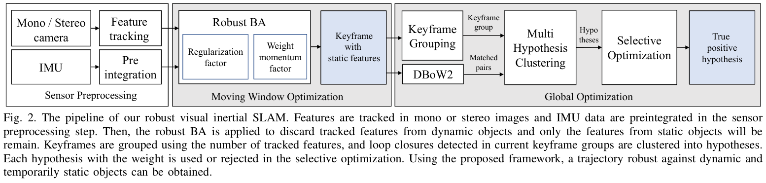
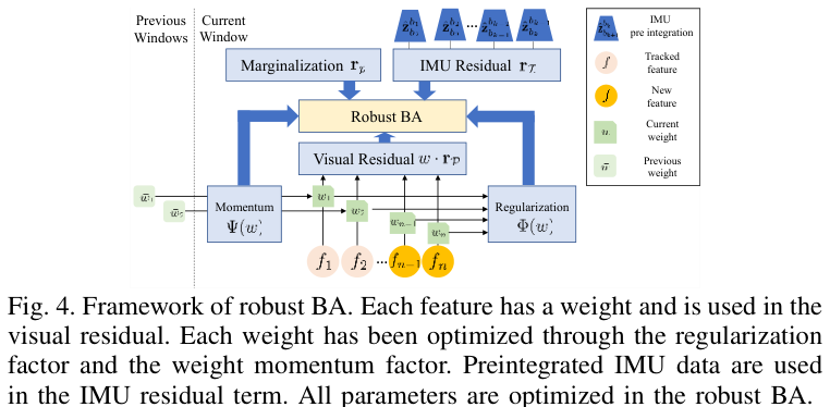
The system tracks features in monocular or stereo images and preintegrates IMU measurements. A sliding window jointly estimates keyframe poses, velocities, inertial biases, and feature depths. Robust bundle adjustment assigns one weight to each tracked feature across its observations. Keyframes with shared tracks are then grouped; visual place recognition proposes matches, which become weighted hypotheses in global optimization.
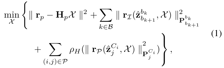
Pose transformations use SE(3). Visual residuals express reprojection errors, while the other objective terms encode inertial observations and information marginalized from previous windows.
Related references: [3], [25].
Robust bundle adjustment
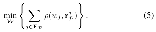
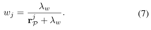
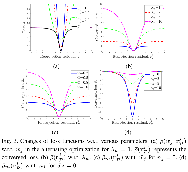
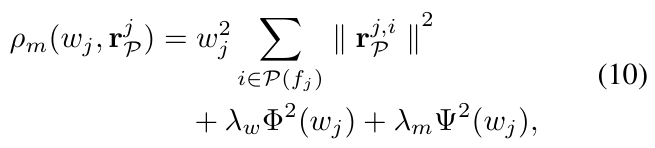
A conventional Huber loss still lets large visual residuals influence the solution. DynaVINS instead multiplies each feature’s accumulated squared reprojection error by its squared weight and adds a penalty that favors weight one. Starting from the inertial pose estimate, it alternates weight updates with state optimization. For the regularization-only objective, the optimal weight equals the regularization strength divided by that strength plus the feature’s accumulated error.
The resulting converged loss saturates for high-error features. Crucially, a feature is not permanently discarded at the first iteration: its weight can recover as the pose estimate improves. Increasing regularization makes the optimization more tolerant of residual error but also admits more influence from dynamic features.
Related references: [21], [22], [23], [24].
Equations 1–8





Keeping useful feature history
Aggressive motion can make inertial preintegration temporarily inaccurate, causing good static features to receive high reprojection errors. A momentum penalty discourages a tracked feature’s current weight from departing from its previous weight; its influence grows with the number of previous optimizations. This retains trusted features and keeps long-tracked outliers weak even if their instantaneous errors fall.
In stereo mode, weights apply to cross-time reprojections. Same-time stereo reprojection is used for depth estimation, since it is not changed by an object’s motion between frames. Its image measurements can still become unreliable in low light.
Equations 9–11


Grouping keyframes and loop-closure hypotheses
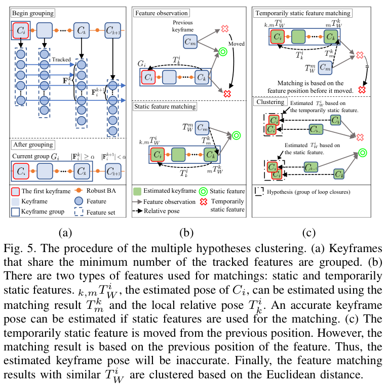
Adjacent keyframes form a group while enough features remain tracked from the group’s first frame. DBoW2 proposes up to three earlier matching frames per current frame. Each match implies a pose for the current group’s first frame, using the local relative motion within the group. Matches with nearby inferred poses are clustered together.
The two largest clusters are retained as competing hypotheses to limit computation. Static and relocated objects can support different clusters, but clustering alone does not identify which one is correct. This construction assumes that relative motion within the current group is sufficiently accurate.
Related references: [25].
Equations 12–14



Selective global optimization
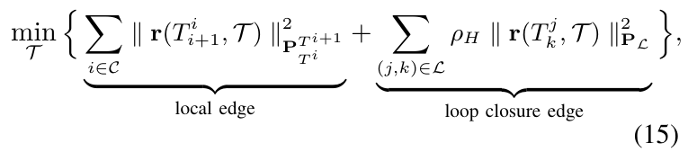
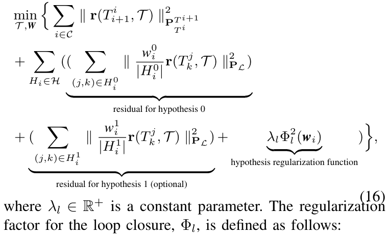
The pose graph combines local motion edges with loop-closure groups. Each of a group’s two hypotheses has a shared weight, and each residual is multiplied by that weight divided by the number of matches before its norm is squared. A regularizer favors a total hypothesis weight near one; inconsistent groups can instead receive low weights for both candidates.
Alternating optimization updates trajectory poses and hypothesis weights. Persistent false matches therefore share a decision instead of adding many independently weighted constraints. Clustering is repeated after pose updates, because the inferred hypothesis positions change with the optimized trajectory.
Related references: [16], [21].
Equations 15–17

Datasets and evaluation design
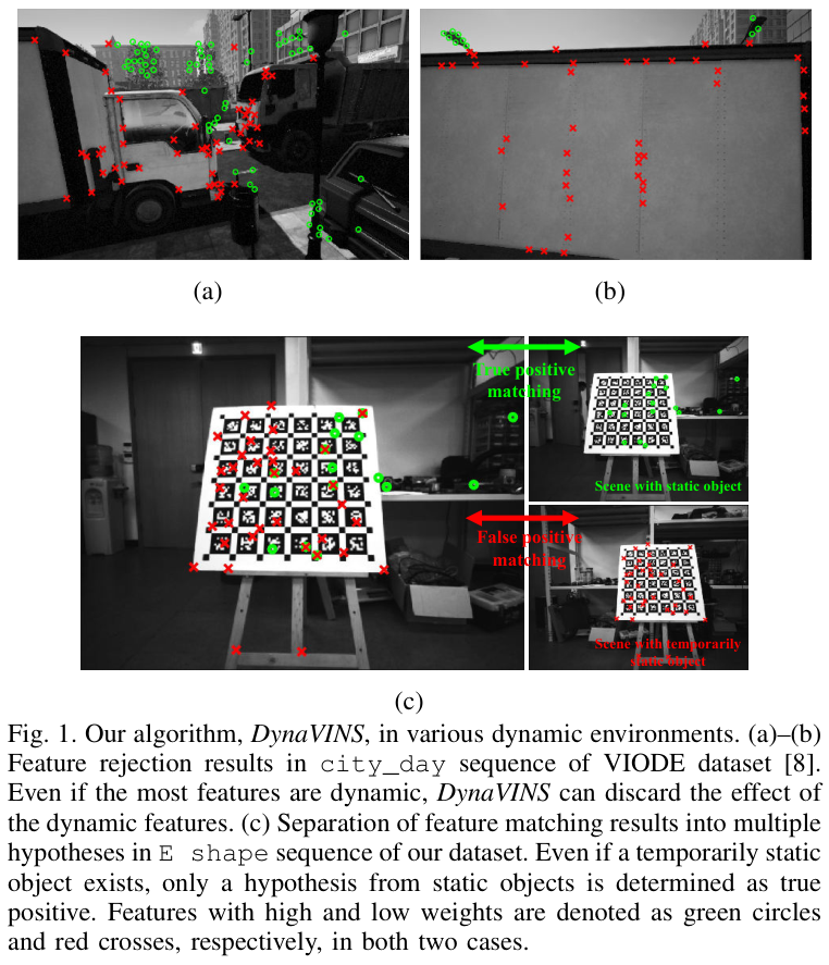
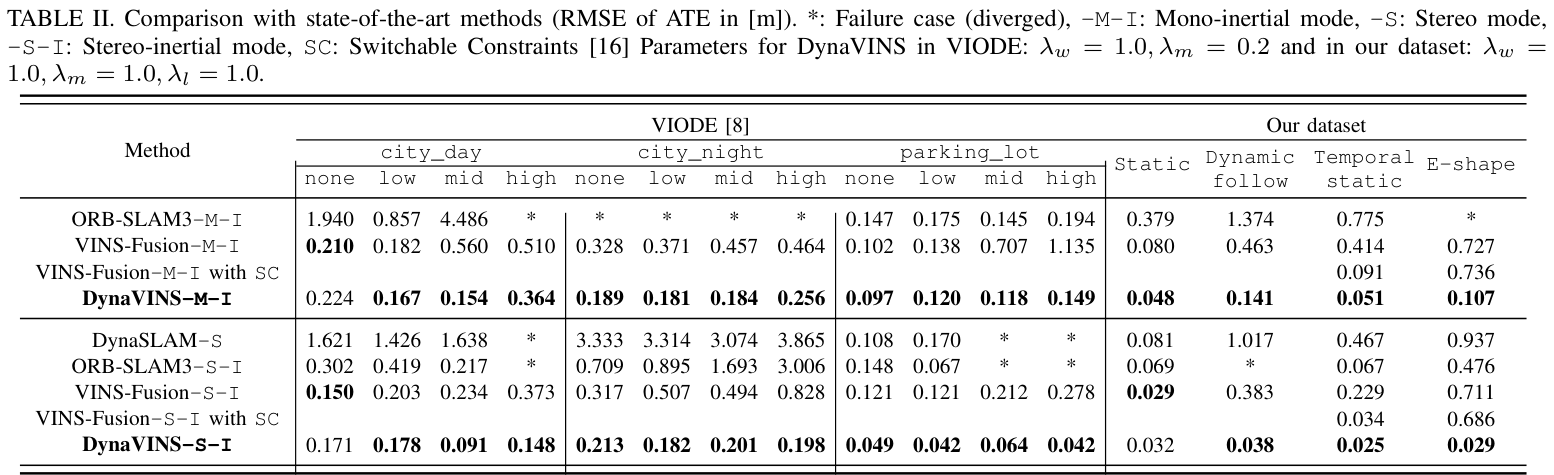
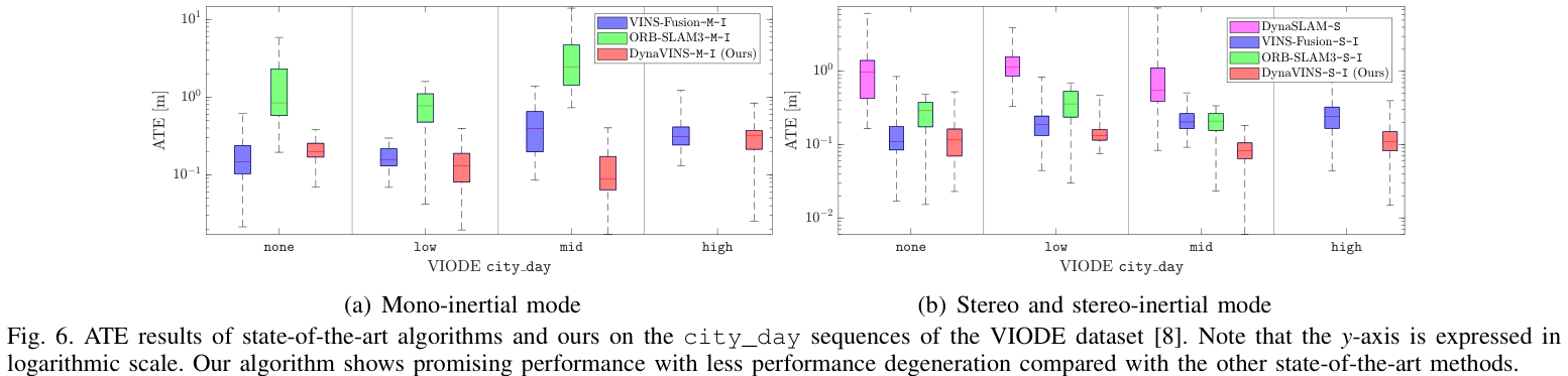
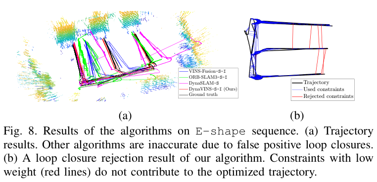
VIODE supplies simulated city_day, city_night, and parking_lot sequences with four levels of moving-object density, including major visual occlusions. Four additional real sequences test a static scene, following a moving occluder, an object relocated between observations, and an E-shaped path with a moved checkerboard that induces repeated false loop closures.
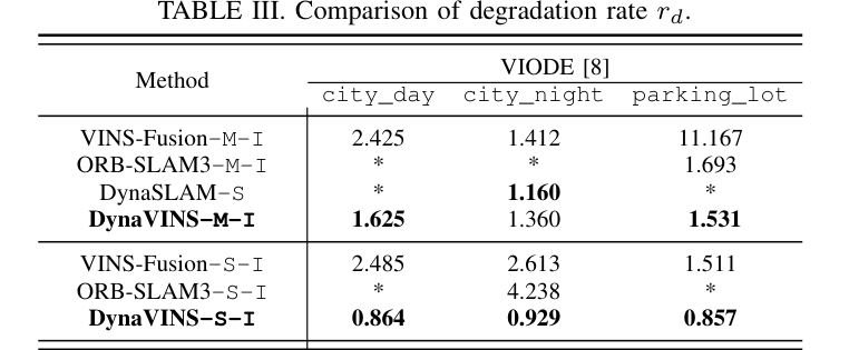
Accuracy is reported as RMSE of aligned absolute trajectory error. Degradation is the high-dynamics error divided by the no-dynamics error. Mono-inertial and stereo-inertial modes are compared with VINS-Fusion and ORB-SLAM3; DynaSLAM uses stereo vision without an IMU, so that comparison does not isolate the algorithm from the sensor advantage. Hyperparameters also differ between simulated and real datasets.
Accuracy, ablations, and runtime
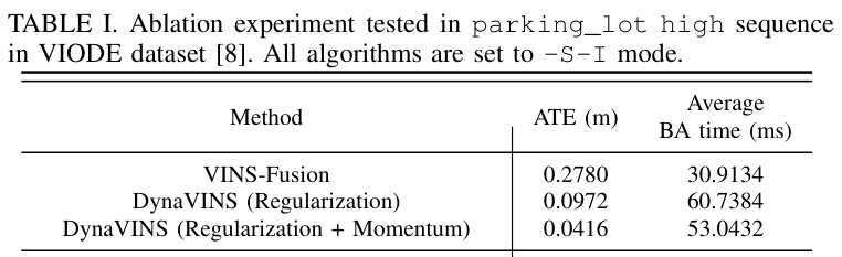
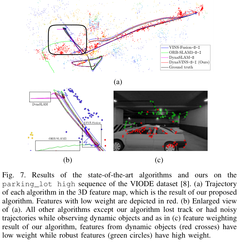
On parking_lot high, the stereo-inertial ablation reduces ATE from 0.2780 m for VINS-Fusion to 0.0972 m with regularization and 0.0416 m with regularization plus momentum. Average bundle-adjustment time rises from 30.91 ms to 60.74 ms for regularization alone, then falls to 53.04 ms with momentum. The latter improves efficiency within DynaVINS while remaining slower than the baseline.
Across VIODE, DynaVINS generally remains accurate as moving-object density increases, including settings in which comparison methods diverge. Its stereo-inertial high/none degradation ratios are 0.864, 0.929, and 0.857 for city_day, city_night, and parking_lot. Ratios below one describe these particular sequence comparisons; they do not establish that more moving objects improve localization generally.
The real E-shape sequence tests persistent false loop closures. Stereo-inertial ATE is 0.029 m for DynaVINS, versus 0.711 m for VINS-Fusion and 0.686 m after adding switchable constraints. Its mono-inertial result is 0.107 m. DynaVINS is not best in every static or low-dynamics case. Original tables retain all results, divergence markers, sensor modes, and parameter settings.
Related references: [3], [5], [8], [9], [16].
Scope and limitations
The method relies on useful inertial priors, adequate local trajectory estimates for hypothesis clustering, and surviving visual information. Its fixed top-two hypothesis selection can discard smaller alternatives. The real tests use four designed sequences, including a feature-rich checkerboard; they are targeted demonstrations rather than broad evidence across uncontrolled deployments.
The reported timing is bundle-adjustment time, not an end-to-end latency guarantee. The authors identify speed improvements and extension to LiDAR–visual–inertial SLAM as future work. The authors’ code and dataset information accompany the paper.