Overview
At a glance
Intuition. A larger network costs more to train on each token. With a fixed budget, increasing its size therefore leaves fewer opportunities to learn from examples. The useful question is which combination of model size and training amount gives the best final predictions, rather than which model can fit in memory.
Reading the math. N is the number of parameters and D the number of training tokens. The rough cost model C ≈ 6ND makes the tradeoff concrete: at the same C, doubling N leaves room for roughly half as many tokens. The fitted recommendation instead doubles both N and D when compute grows roughly fourfold.
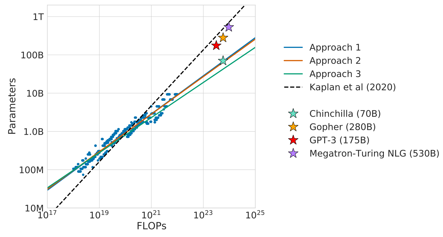
For a fixed training-compute budget, the study asks how to divide resources between model parameters and training tokens. More than 400 training runs and three fitting methods favor increasing both quantities at roughly equal rates as compute grows. A 70B-parameter model trained on 1.4T tokens, Chinchilla, then outperforms the 280B Gopher across most tested tasks at a similar training budget. The result is an empirical allocation rule for the studied dense autoregressive transformers and training regime, rather than a universal law for every architecture, dataset, or deployment objective.
1 Introduction
Training the largest model possible is not necessarily the best use of a fixed budget. The paper minimizes final loss over parameter count N and token count D subject to a compute constraint. Earlier practice often increased parameters while keeping tokens near 300B; these experiments instead predict smaller models trained longer. The large-scale comparison supports that prediction and makes downstream inference cheaper because the resulting model is smaller. Training-compute optimality, inference cost, and total lifetime cost are different objectives; only the first is directly fitted here.
The principal prior scaling comparison is [Kaplan et al., 2020]; the large-model baseline follows the Gopher study cited in the source bibliography.
| Model | Size ( Parameters) | Training Tokens |
|---|---|---|
| LaMDA (Thoppilan et al., 2022) | 137 Billion | 168 Billion |
| GPT-3 (Brown et al., 2020) | 175 Billion | 300 Billion |
| Jurassic (Lieber et al., 2021) | 178 Billion | 300 Billion |
| Gopher (Rae et al., 2021) | 280 Billion | 300 Billion |
| MT-NLG 530B (Smith et al., 2022) | 530 Billion | 270 Billion |
| Chinchilla | 70 Billion | 1.4 Trillion |
Equation 1
| (1) |
2 Related Work
Large language models.
Dense and mixture-of-experts language models had improved many benchmarks by scaling parameters, while their computational requirements and demand for high-quality data grew. This study investigates the parameter–data trade-off for dense models. Its conclusions should not be transferred unchanged to routed models.
Modelling the scaling behavior.
The comparison with earlier scaling work emphasizes two experimental differences: matching the learning-rate decay horizon to the actual training duration, and including substantially larger models in the fitting corpus. Intermediate checkpoints on a long decay schedule can overestimate the loss achievable by a shorter, correctly scheduled run. The paper also observes curvature that makes extrapolation from only tiny models unreliable. These are empirical explanations for differing allocation exponents, rather than a mathematical refutation of every previous scaling result.
Estimating hyperparameters for large models.
The study varies model size and training duration while choosing other hyperparameters using existing heuristics. Learning rate, batch size, optimizer, and depth-to-width ratio can also affect the frontier. The selected architectures are slightly shallower than one cited recommendation to improve wall-clock efficiency on the authors’ hardware.
Improved model architectures.
Conditional computation and retrieval are alternative ways to improve performance without simply increasing dense parameter count. The cited routed-model scaling studies often fix token count, while retrieval exposes models to additional text. These comparisons motivate studying data allocation but do not establish the same fitted scaling exponents for these different architectures.
3 Estimating the optimal parameter/training tokens allocation
All three approaches train families of models with varying sizes and durations, then estimate a compute-efficient frontier. They assume power-law scaling for extrapolation. Agreement among different fits strengthens the observed trend, while the shared training setup and finite scale range remain common limitations.
3.1 Approach 1: Fix model sizes and vary number of training tokens
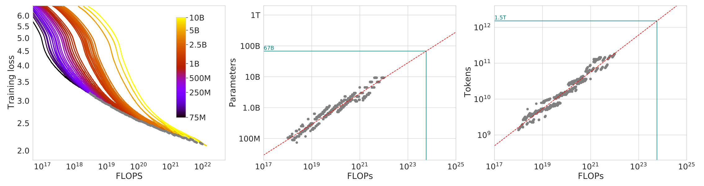
Approach 1 smooths and interpolates training curves for fixed parameter counts with four decay horizons. At 1,500 logarithmically spaced compute values it selects the lowest observed interpolated loss, records the winning model and token count, and fits their scaling with compute. The fitted exponents are approximately 0.50 for both parameters and tokens. Selected points lie near the ends of runs, supporting decay schedules matched to the intended horizon. The envelope is estimated from a finite family, not an exhaustive optimization over all training recipes.
3.2 Approach 2: IsoFLOP profiles
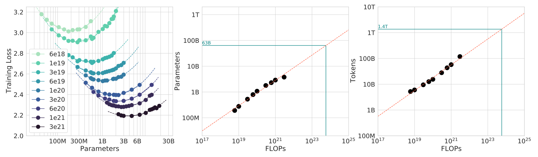
Approach 2 fixes nine compute budgets and varies model size, which determines the available token budget. A parabola fitted to each IsoFLOP loss profile estimates its best parameter count. Power-law fits through those minima yield exponents 0.49 for model size and 0.51 for tokens. Matching each run’s cosine schedule to its own duration avoids treating incompletely decayed intermediate checkpoints as equivalent final models.
3.3 Approach 3: Fitting a parametric loss function
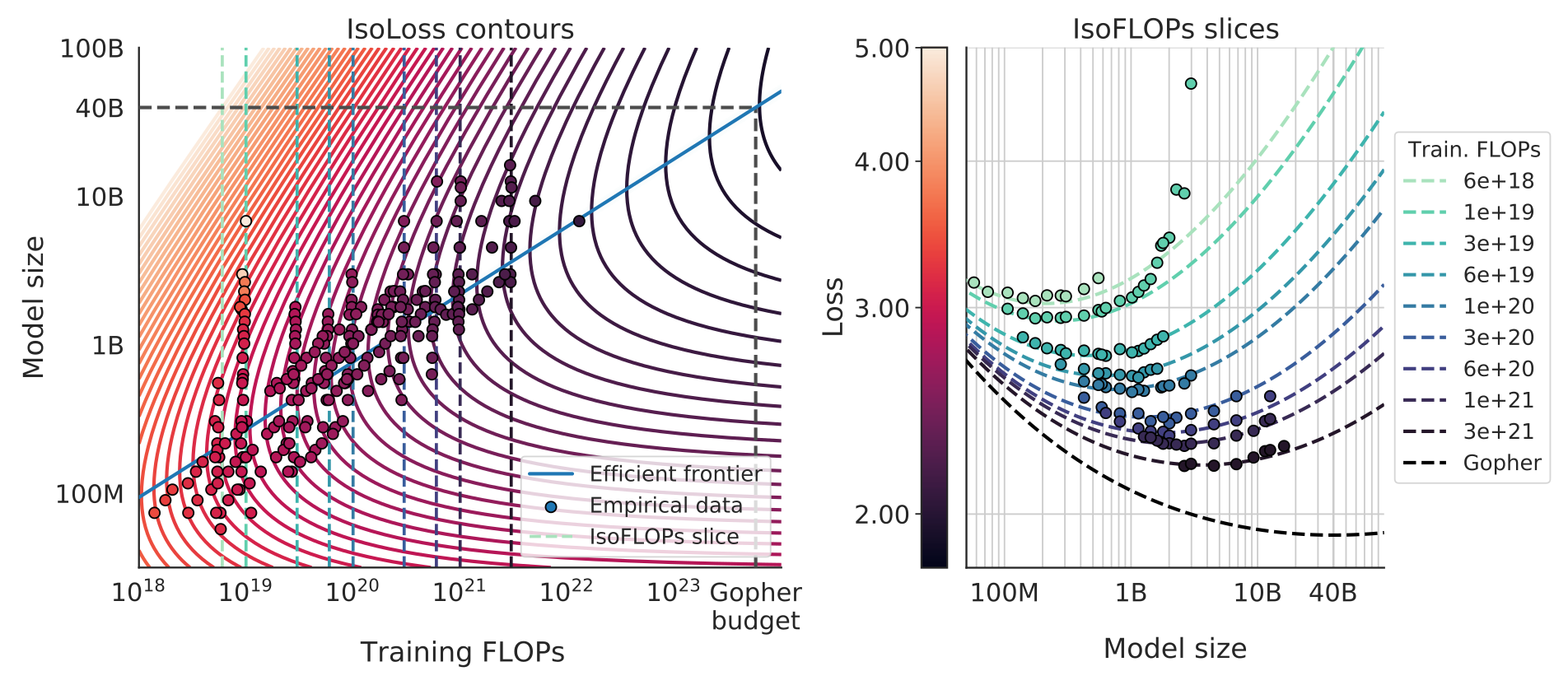
Approach 3 fits loss as an irreducible term plus separate parameter-limited and token-limited power-law terms. The decomposition is a useful empirical model: it is not a proof that finite transformer approximation and optimization errors must separate exactly in this way.
Equation 2
| (2) |
Model fitting.
The five coefficients are fitted to observed log losses using a Huber objective and L-BFGS, with a grid of initializations to reduce sensitivity to local optima. A small Huber threshold limits the influence of poor-fitting runs. Robust fitting changes which regions influence the prediction; it does not eliminate extrapolation error.
Equation 3
| (3) |
Efficient frontier.
Minimizing the fitted loss under the approximation C≈6ND gives an analytic compute frontier. The resulting exponents are 0.46 for parameters and 0.54 for tokens, favoring even smaller, longer-trained models than the other methods at high budgets. The optimum balances the marginal benefits of the fitted parameter and data terms.
Equation 4
| (4) |
3.4 Optimal model scaling
The three estimated exponent pairs all favor near-equal scaling, unlike the earlier 0.73/0.27 allocation. Their exact predictions differ, particularly when extrapolating far beyond observed compute. The parametric fit discounts many small-budget points and predicts smaller optimal models because of observed frontier curvature. All confidence ranges and projected budgets remain in Tables 2–3. The source’s rounded point estimates do not always fall inside their printed bootstrap intervals, and nearby prose gives some budgets different from Table 3; these are preserved rather than silently reconciled. The supported conclusion is the broad allocation trend, with uncertainty in exact large-scale prescriptions.
| Approach | Coeff. where | Coeff. where |
|---|---|---|
| 1. Minimum over training curves | ||
| 2. IsoFLOP profiles | ||
| 3. Parametric modelling of the loss | ||
| Kaplan et al. (2020) | 0.73 | 0.27 |
.
| Parameters | FLOPs | FLOPs (in Gopher unit) | Tokens |
|---|---|---|---|
| 400 Million | 1.92e+19 | 8.0 Billion | |
| 1 Billion | 1.21e+20 | 20.2 Billion | |
| 10 Billion | 1.23e+22 | 205.1 Billion | |
| 67 Billion | 5.76e+23 | 1.5 Trillion | |
| 175 Billion | 3.85e+24 | 3.7 Trillion | |
| 280 Billion | 9.90e+24 | 5.9 Trillion | |
| 520 Billion | 3.43e+25 | 11.0 Trillion | |
| 1 Trillion | 1.27e+26 | 21.2 Trillion | |
| 10 Trillion | 1.30e+28 | 216.2 Trillion |
4 Chinchilla
The analysis predicts a40–70B model for Gopher’s training budget. The authors choose70B and train on 1.4T tokens, balancing dataset and hardware considerations. This tests one large-scale allocation rather than locating the exact global optimum. A fourfold smaller model also reduces memory and inference cost.
4.1 Model and training details
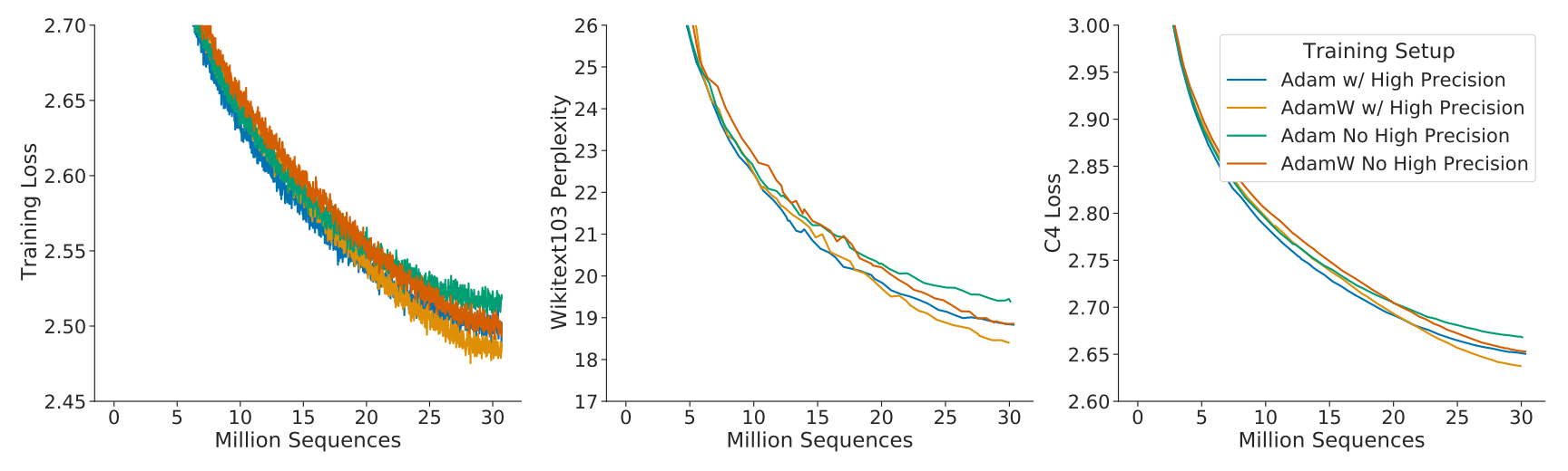
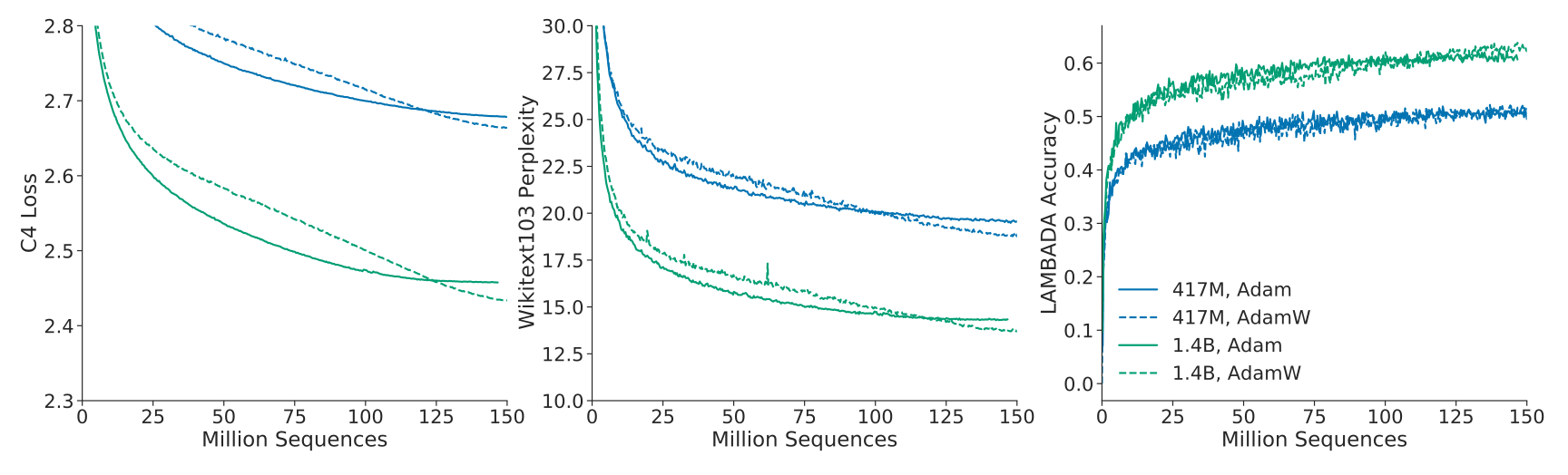
Chinchilla broadly follows Gopher’s architecture and dataset, but the comparison changes more than N and D. It adjusts sampling proportions, uses AdamW instead of Adam, modifies SentencePiece normalization, and retains float32 master weights while computing forward and backward passes in bfloat16. Table 4 preserves the architecture, learning-rate, and batch-size settings. Appendix G ablates some optimizer/precision changes. These differences limit a purely causal attribution of the whole performance gain to token allocation alone.
| Model | Layers | Number Heads | Key/Value Size | dmodel | Max LR | Batch Size |
|---|---|---|---|---|---|---|
| Gopher 280B | 80 | 128 | 128 | 16,384 | 3M 6M | |
| Chinchilla 70B | 80 | 64 | 128 | 8,192 | 1.5M 3M |
4.2 Results
Evaluation covers language modeling, reading comprehension, question answering, common sense,57 MMLU subjects, and 62 BIG-bench tasks, following much of Gopher’s protocol. The complete task groups and source results remain available. Cross-paper comparisons require matching prompts, splits, and shot counts.
| # Tasks | Examples | |
|---|---|---|
| Language Modelling | 20 | WikiText-103, The Pile: PG-19, arXiv, FreeLaw, |
| Reading Comprehension | 3 | RACE-m, RACE-h, LAMBADA |
| Question Answering | 3 | Natural Questions, TriviaQA, TruthfulQA |
| Common Sense | 5 | HellaSwag, Winogrande, PIQA, SIQA, BoolQ |
| MMLU | 57 | High School Chemistry, Astronomy, Clinical Knowledge, |
| BIG-bench | 62 | Causal Judgement, Epistemic Reasoning, Temporal Sequences, |
4.2.1 Language modelling
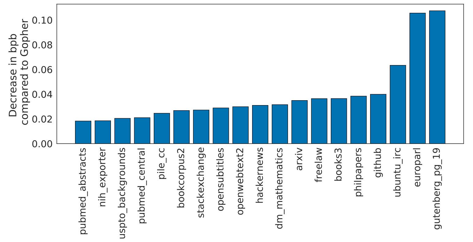
Chinchilla improves bits per byte over Gopher on every reported Pile subset and improves WikiText-103 perplexity from 7.75 to 7.16. Jurassic-1 remains better on two Pile subsets. The authors explicitly warn that more training data can increase train/test overlap, so these language-modeling gains alone are insufficient evidence of uncontaminated generalization.
4.2.2 MMLU
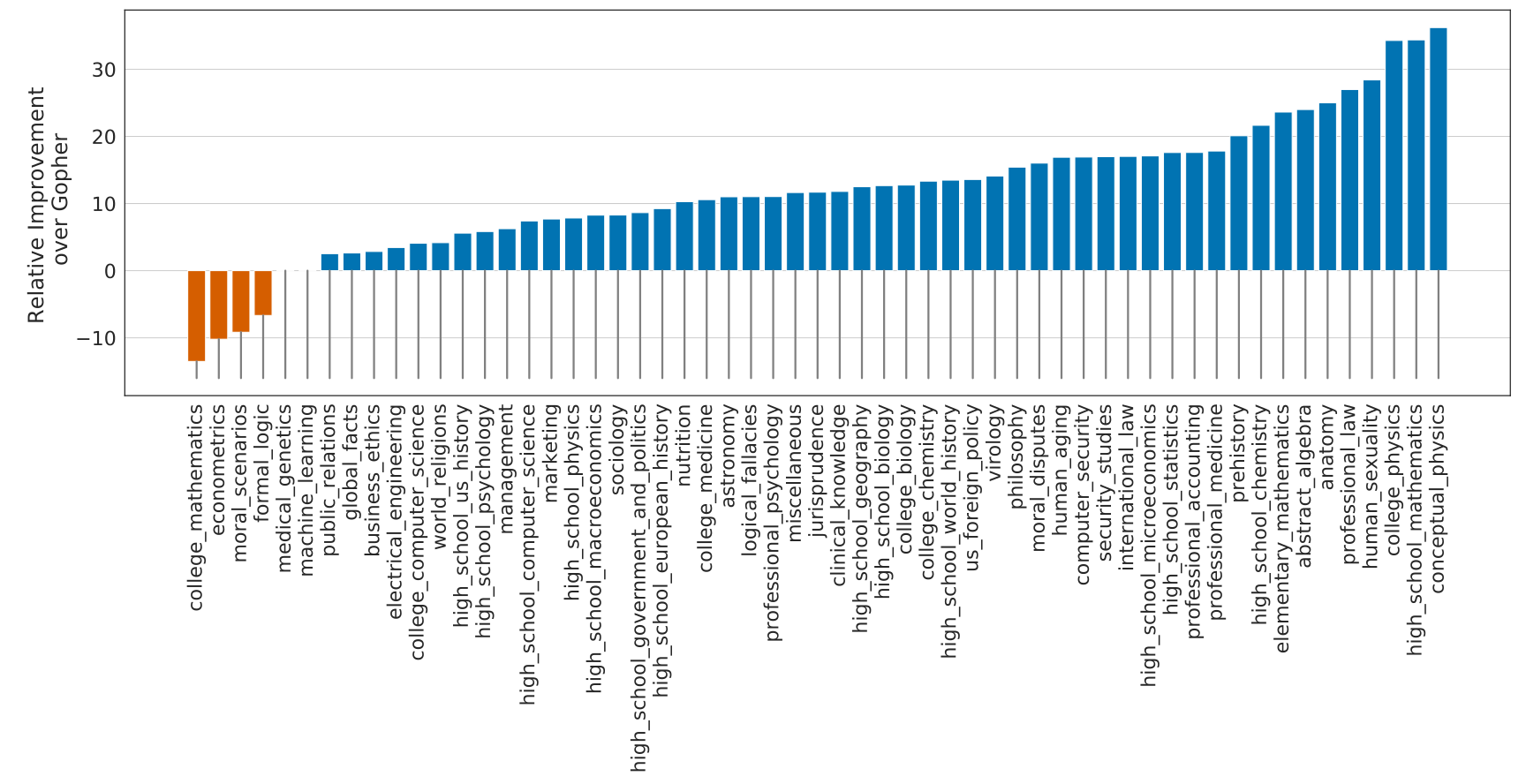
The main results table reports 67.6% average five-shot MMLU accuracy versus 60.0% for Gopher, an increase of 7.6 percentage points. Chinchilla improves51 of 57 subjects, ties two, and declines on four. The abstract instead prints 67.5%; both source occurrences remain unchanged. The forecasts shown are historical comparisons, not current benchmark records.
| Random | 25.0% |
|---|---|
| Average human rater | 34.5% |
| GPT-3 5-shot | 43.9% |
| Gopher 5-shot | 60.0% |
| Chinchilla 5-shot | 67.6% |
| Average human expert performance | 89.8% |
| June 2022 Forecast | 57.1% |
| June 2023 Forecast | 63.4% |
4.2.3 Reading comprehension
Chinchilla improves LAMBADA final-word accuracy to 77.4% and improves both RACE tasks by over ten percentage points relative to Gopher. The source warns that GPT-3 and MT-NLG use different RACE prompts, so their numbers are not directly comparable to the Gopher–Chinchilla pair.
| Chinchilla | Gopher | GPT-3 | MT-NLG 530B | |
|---|---|---|---|---|
| LAMBADA Zero-Shot | 77.4 | 74.5 | 76.2 | 76.6 |
| RACE-m Few-Shot | 86.8 | 75.1 | 58.1 | - |
| RACE-h Few-Shot | 82.3 | 71.6 | 46.8 | 47.9 |
4.2.4 BIG-bench
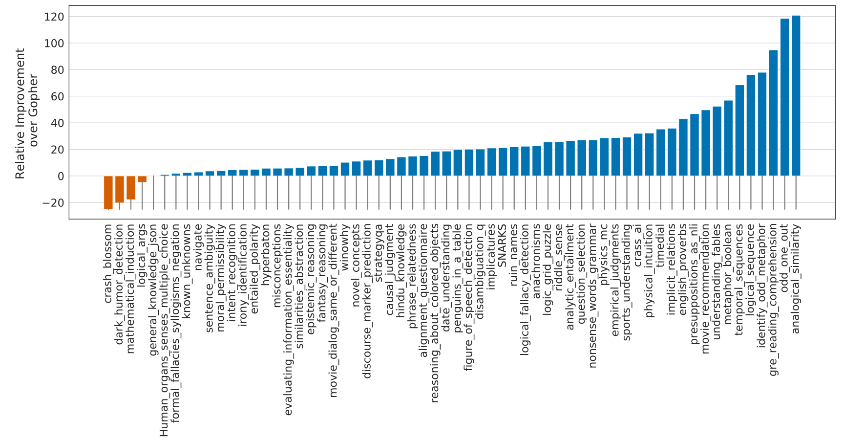
Across the62 selected BIG-bench tasks, mean accuracy rises from 54.4% to 65.1%, a 10.7-percentage-point gain. Four tasks decline. Figures and Appendix H retain the per-task outcomes rather than implying uniform improvement.
4.2.5 Common sense
On the five common-sense tasks, Chinchilla matches or improves Gopher; PIQA is a tie at 81.8%, despite the prose’s broader outperformance claim. TruthfulQA improves substantially under the stated shot settings. These results show that improved pretraining can help this evaluation, without establishing that factuality, truthfulness, or safety always improves with lower language-modeling loss.
| Chinchilla | Gopher | GPT-3 | MT-NLG 530B | Supervised SOTA | |
|---|---|---|---|---|---|
| HellaSWAG | 80.8% | 79.2% | 78.9% | 80.2% | 93.9% |
| PIQA | 81.8% | 81.8% | 81.0% | 82.0% | 90.1% |
| Winogrande | 74.9% | 70.1% | 70.2% | 73.0% | 91.3% |
| SIQA | 51.3% | 50.6% | - | - | 83.2% |
| BoolQ | 83.7% | 79.3% | 60.5% | 78.2% | 91.4% |
4.2.6 Closed-book question answering
Closed-book Natural Questions and TriviaQA generally improve over Gopher across the retained settings. Filtered and unfiltered TriviaQA use different splits and comparison systems, including an open-book retriever model. Table 9 is the comparison record: the prose’s Gopher five-shot Natural Questions value differs from that table, so the table and original wording are retained without substituting a guessed correction.
| Method | Chinchilla | Gopher | GPT-3 | SOTA (open book) | |
|---|---|---|---|---|---|
| Natural Questions (dev) | 0-shot | 16.6% | 10.1% | 14.6% | 54.4% |
| 5-shot | 31.5% | 24.5% | - | ||
| 64-shot | 35.5% | 28.2% | 29.9% | ||
| TriviaQA (unfiltered, test) | 0-shot | 67.0% | 52.8% | 64.3 % | - |
| 5-shot | 73.2% | 63.6% | - | ||
| 64-shot | 72.3% | 61.3% | 71.2% | ||
| TriviaQA (filtered, dev) | 0-shot | 55.4% | 43.5% | - | 72.5% |
| 5-shot | 64.1% | 57.0% | - | ||
| 64-shot | 64.6% | 57.2% | - |
4.2.7 Gender bias and toxicity
The paper evaluates a limited selection of gender/coreference and unprompted-toxicity behaviors. It explicitly describes these checks as incomplete. Better benchmark averages do not eliminate the risks inherited from training data or establish downstream deployment safety.
Gender bias.
Winogender coreference accuracy improves from 71.4% to 78.3%, but improvements differ across male, female, and neutral pronouns. Accuracy on stereotype-contradicting examples also improves unevenly. The retained group breakdown reveals residual disparities; aggregate improvement does not demonstrate absence of gender bias.
| Chinchilla | Gopher | |
|---|---|---|
| All | 78.3% | 71.4% |
| Male | 71.2% | 68.0% |
| Female | 79.6% | 71.3% |
| Neutral | 84.2% | 75.0% |
| Chinchilla | Gopher | |
|---|---|---|
| Male gotcha | 62.5% | 59.2% |
| Male not gotcha | 80.0% | 76.7% |
| Female gotcha | 76.7% | 66.7% |
| Female not gotcha | 82.5% | 75.8% |
Sample toxicity.
The authors generate25,000 unprompted samples and compare PerspectiveAPI scores. Mean toxicity is 0.087 for Chinchilla versus 0.081 for Gopher, with similarly close medians and 95th percentiles. The study interprets these differences as negligible. This particular classifier-based, unconditional test neither proves all toxicity risks unchanged nor supports a broad claim that Chinchilla is less toxic.
5 Discussion & Conclusion
The main evidence supports reallocating a fixed training budget toward smaller models and more tokens in this regime. Limitations include only one large-scale Chinchilla–Gopher comparison, incomplete intermediate-scale tests, power-law extrapolation, and observed curvature. The scaling runs study less-than-one-epoch training; this should not be confused with every subset in the final mixture, whose epoch counts appear in Appendix A. High-quality dataset expansion and overlap checks are important practical implications. The paper’s speculative discussion of future datasets is separate from an experimentally established universal data-quality law.
6 Acknowledgements
The acknowledgements credit colleagues for manuscript feedback, technical discussions, and JAX/XLA assistance.
Appendix
Appendix A Training dataset
The exact MassiveText mixture, document counts, sampling proportions, and effective epochs remain in Table A1. Chinchilla adjusts the mixture relative to Gopher. Although the scaling analysis is discussed as a single-pass regime, the final 1.4T-token mixture revisits MassiveWeb and Wikipedia, reported at 1.24 and 3.40 epochs respectively.
| Disk Size | Documents | Sampling proportion | Epochs in 1.4T tokens | |
|---|---|---|---|---|
| MassiveWeb | 1.9 TB | 604M | 45% (48%) | 1.24 |
| Books | 2.1 TB | 4M | 30% (27%) | 0.75 |
| C4 | 0.75 TB | 361M | 10% (10%) | 0.77 |
| News | 2.7 TB | 1.1B | 10% (10%) | 0.21 |
| GitHub | 3.1 TB | 142M | 4% (3%) | 0.13 |
| Wikipedia | 0.001 TB | 6M | 1% (2%) | 3.40 |
Appendix B Optimal cosine cycle length
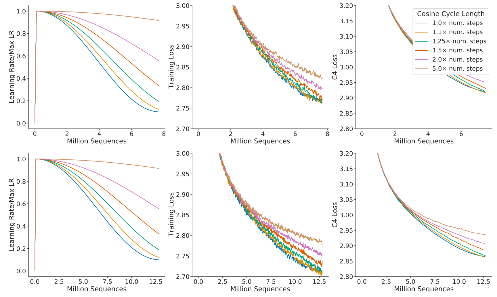
Cosine schedules much longer than the intended training horizon give worse final loss. The grid compares six cycle lengths at two target durations and finds clear degradation when overshooting by more than 25%. This supports the chosen horizon-matching convention under the examined settings, rather than proving one schedule optimal for every budget and optimizer.
Appendix C Consistency of scaling results across datasets
Additional IsoFLOP experiments on C4 and GitHub code estimate near-equal parameter/token scaling, with pairs 0.50/0.50 and 0.53/0.47. These replications broaden the dataset evidence. Two related corpora with the same tokenizer do not establish independence from all possible data distributions or repeated-epoch regimes.
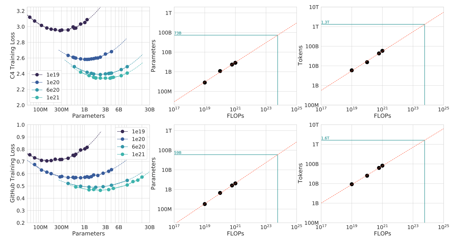
| Approach | Coef. where | Coef. where |
|---|---|---|
| C4 | 0.50 | 0.50 |
| GitHub | 0.53 | 0.47 |
| Kaplan et al. (2020) | 0.73 | 0.27 |
Appendix D Details on the scaling analyses
D.1 Approach 1: Fixing model sizes and varying training sequences
Approach 1 uses a tenfold cosine learning-rate decay, size-dependent maximum learning rates, and a ten-step Gaussian smoothing window. These details determine the envelope used for fitting and should be matched when reproducing the allocation estimates.
D.2 Approach 3: Parametric fitting of the loss
The appendix motivates the fitted loss through an expected-risk decomposition and specifies its robust numerical fitting. The decomposition is exact as an algebraic addition/subtraction of risks, while the separable power laws subsequently assigned to those terms are modeling assumptions.
Equation 5
| (5) |
Loss decomposition.
The argument separates Bayes risk, finite-model approximation error, and the suboptimality of a finite-data, single-pass stochastic training procedure. Equations 6 and 8 print positive expected log probability while minimizing it; conventional cross-entropy requires its negative. The original equations are retained as printed. The surrounding entropy discussion and positive loss fits should not be implemented by minimizing that printed sign without checking the intended negative-log-likelihood convention.
Equations 6–9
| (6) |
| (7) |
| (8) |
| (9) |
Expected forms of the loss terms.
The authors motivate power-law forms from simpler approximation and stochastic-optimization results, then fit parameter and data exponents 0.34 and 0.28 with E=1.69, A=406.4, and B=410.7. The cited simpler-model rates do not establish these exact transformer exponents or exact N–D separability. This empirical fit does not uniquely identify language’s intrinsic dimension.
Equation 10
| (10) |
Fitting the decomposition to data.
Log-sum-exp parameterization keeps the loss coefficients positive. L-BFGS searches from a specified initialization grid and uses Huber threshold10⁻³. Larger thresholds overemphasize the small-compute regime in these fits; smaller ones reportedly make little difference. Retaining the objective and initialization grid supports reproduction.
Equation 11
| (11) |
D.3 Predicted compute optimal frontier for all three methods
Table A3 and Figure A3 retain the alternative methods’ projected budgets. One source entry is internally inconsistent: Approach 3 lists175B parameters,12.0T tokens, and 1.26×10²⁴ FLOPs, whereas6ND is about 1.26×10²⁵. This appears to be a table exponent issue; the edition preserves it and does not infer a software error. Long-range projections remain uncertain even where arithmetic is consistent.
| Approach 2 | Approach 3 | |||
|---|---|---|---|---|
| Parameters | FLOPs | Tokens | FLOPs | Tokens |
| 400 Million | 1.84e+19 | 7.7 Billion | 2.21e+19 | 9.2 Billion |
| 1 Billion | 1.20e+20 | 20.0 Billion | 1.62e+20 | 27.1 Billion |
| 10 Billion | 1.32e+22 | 219.5 Billion | 2.46e+22 | 410.1 Billion |
| 67 Billion | 6.88e+23 | 1.7 Trillion | 1.71e+24 | 4.1 Trillion |
| 175 Billion | 4.54e+24 | 4.3 Trillion | 1.26e+24 | 12.0 Trillion |
| 280 Billion | 1.18e+25 | 7.1 Trillion | 3.52e+25 | 20.1 Trillion |
| 520 Billion | 4.19e+25 | 13.4 Trillion | 1.36e+26 | 43.5 Trillion |
| 1 Trillion | 1.59e+26 | 26.5 Trillion | 5.65e+26 | 94.1 Trillion |
| 10 Trillion | 1.75e+28 | 292.0 Trillion | 8.55e+28 | 1425.5 Trillion |
.
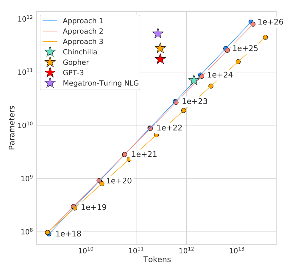
D.4 Small-scale comparison to Kaplan et al. (2020)
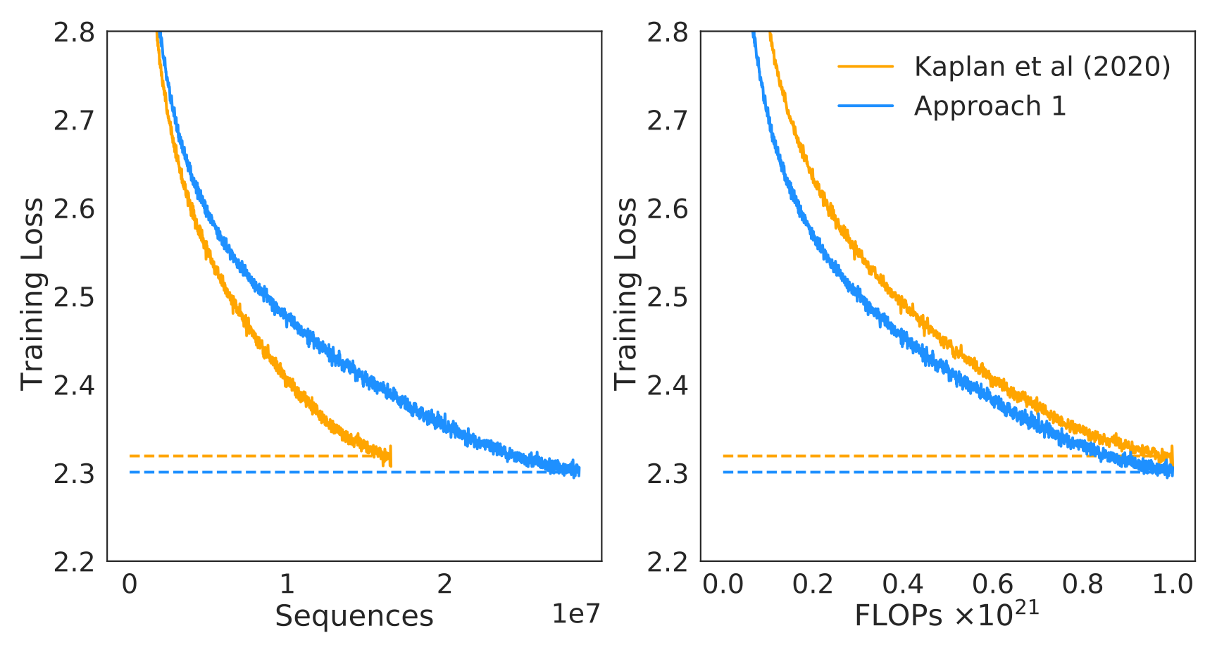
At10²¹ FLOPs, the study directly compares a 2.80B model near its prediction with a 4.74B model near the earlier scaling prediction, holding the depth-to-width ratio and key training choices fixed. The smaller model has the better final loss. This is additional controlled evidence at that budget, rather than validation of every extrapolated budget in the tables.
Appendix E Curvature of the FLOP-loss frontier
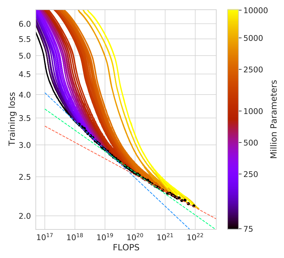
Fitting different thirds of the loss-efficient envelope reveals curvature. The paper’s principal allocation fits do not model it explicitly. Consequently, extrapolating a single straight power law from only the smallest runs can bias the predicted optimal model size.
Appendix F FLOPs computation
The original nested accounting list is preserved in full, including embeddings, attention projections/logits/softmax/reductions/output projection, feed-forward blocks, and final logits. It counts a multiply-accumulate as two operations and approximates backward computation as twice forward computation. Table A4 compares this calculation with 6ND. The source also reports a revised Gopher compute estimate, so budget values should be interpreted with their stated counting convention.
- •
Embeddings
- –
- –
- •
Attention (Single Layer)
- –
Key, query and value projections:
- –
Key @ Query logits:
- –
Softmax:
- –
Softmax @ query reductions:
- –
Final Linear:
- –
- •
Dense Block (Single Layer)
- –
- –
- •
Final Logits
- –
- –
- •
Total forward pass FLOPs: + logits
| Parameters | num_layers | d_model | ffw_size | num_heads | k/q size | FLOP Ratio (Ours/) |
|---|---|---|---|---|---|---|
| 73M | 10 | 640 | 2560 | 10 | 64 | 1.03 |
| 305M | 20 | 1024 | 4096 | 16 | 64 | 1.10 |
| 552M | 24 | 1280 | 5120 | 10 | 128 | 1.08 |
| 1.1B | 26 | 1792 | 7168 | 14 | 128 | 1.04 |
| 1.6B | 28 | 2048 | 8192 | 16 | 128 | 1.03 |
| 6.8B | 40 | 3584 | 14336 | 28 | 128 | 0.99 |
Appendix G Other differences between Chinchilla and Gopher
The auxiliary comparisons separate some benefits of AdamW and float32 master weights. They show training and downstream differences beyond the parameter–token allocation. These ablations are smaller-scale evidence and do not make the main Chinchilla–Gopher comparison a perfectly isolated two-variable experiment.
Appendix H Results
H.1 The Pile
The complete Pile table retains bits-per-byte values for Chinchilla, Gopher, and Jurassic-1, including the two subsets where Jurassic-1 does better. The train/test-overlap caveat from the main language-modeling section still applies.
| Subset | Chinchilla (70B) | Gopher (280B) | Jurassic-1 (170B) |
|---|---|---|---|
| pile_cc | 0.667 | 0.691 | 0.669 |
| pubmed_abstracts | 0.559 | 0.578 | 0.587 |
| stackexchange | 0.614 | 0.641 | 0.655 |
| github | 0.337 | 0.377 | 0.358 |
| openwebtext2 | 0.647 | 0.677 | - |
| arxiv | 0.627 | 0.662 | 0.680 |
| uspto_backgrounds | 0.526 | 0.546 | 0.537 |
| freelaw | 0.476 | 0.513 | 0.514 |
| pubmed_central | 0.504 | 0.525 | 0.579 |
| dm_mathematics | 1.111 | 1.142 | 1.037 |
| hackernews | 0.859 | 0.890 | 0.869 |
| nih_exporter | 0.572 | 0.590 | 0.590 |
| opensubtitles | 0.871 | 0.900 | 0.879 |
| europarl | 0.833 | 0.938 | - |
| books3 | 0.675 | 0.712 | 0.835 |
| philpapers | 0.656 | 0.695 | 0.742 |
| gutenberg_pg_19 | 0.548 | 0.656 | 0.890 |
| bookcorpus2 | 0.714 | 0.741 | - |
| ubuntu_irc | 1.026 | 1.090 | 0.857 |
H.2 MMLU
All57 MMLU subject scores remain in the table. Their variation—including low mathematics scores, four regressions, and two ties—provides essential context for the high overall mean.
| Task | Chinchilla | Gopher | Task | Chinchilla | Gopher |
|---|---|---|---|---|---|
| abstract_algebra | 31.0 | 25.0 | anatomy | 70.4 | 56.3 |
| astronomy | 73.0 | 65.8 | business_ethics | 72.0 | 70.0 |
| clinical_knowledge | 75.1 | 67.2 | college_biology | 79.9 | 70.8 |
| college_chemistry | 51.0 | 45.0 | college_computer_science | 51.0 | 49.0 |
| college_mathematics | 32.0 | 37.0 | college_medicine | 66.5 | 60.1 |
| college_physics | 46.1 | 34.3 | computer_security | 76.0 | 65.0 |
| conceptual_physics | 67.2 | 49.4 | econometrics | 38.6 | 43.0 |
| electrical_engineering | 62.1 | 60.0 | elementary_mathematics | 41.5 | 33.6 |
| formal_logic | 33.3 | 35.7 | global_facts | 39.0 | 38.0 |
| high_school_biology | 80.3 | 71.3 | high_school_chemistry | 58.1 | 47.8 |
| high_school_computer_science | 58.0 | 54.0 | high_school_european_history | 78.8 | 72.1 |
| high_school_geography | 86.4 | 76.8 | high_school_gov_and_politics | 91.2 | 83.9 |
| high_school_macroeconomics | 70.5 | 65.1 | high_school_mathematics | 31.9 | 23.7 |
| high_school_microeconomics | 77.7 | 66.4 | high_school_physics | 36.4 | 33.8 |
| high_school_psychology | 86.6 | 81.8 | high_school_statistics | 58.8 | 50.0 |
| high_school_us_history | 83.3 | 78.9 | high_school_world_history | 85.2 | 75.1 |
| human_aging | 77.6 | 66.4 | human_sexuality | 86.3 | 67.2 |
| international_law | 90.9 | 77.7 | jurisprudence | 79.6 | 71.3 |
| logical_fallacies | 80.4 | 72.4 | machine_learning | 41.1 | 41.1 |
| management | 82.5 | 77.7 | marketing | 89.7 | 83.3 |
| medical_genetics | 69.0 | 69.0 | miscellaneous | 84.5 | 75.7 |
| moral_disputes | 77.5 | 66.8 | moral_scenarios | 36.5 | 40.2 |
| nutrition | 77.1 | 69.9 | philosophy | 79.4 | 68.8 |
| prehistory | 81.2 | 67.6 | professional_accounting | 52.1 | 44.3 |
| professional_law | 56.5 | 44.5 | professional_medicine | 75.4 | 64.0 |
| professional_psychology | 75.7 | 68.1 | public_relations | 73.6 | 71.8 |
| security_studies | 75.9 | 64.9 | sociology | 91.0 | 84.1 |
| us_foreign_policy | 92.0 | 81.0 | virology | 53.6 | 47.0 |
| world_religions | 87.7 | 84.2 |
H.3 Winogender Setup
The Winogender procedure compares probabilities of two candidate referents after a sentence and a coreference prompt. Each example is evaluated with female, male, and neutral pronouns. This tests one controlled coreference behavior, rather than the full range of gender-related outputs or intersectional bias.
H.4 BIG-bench
The complete62-task BIG-bench comparison preserves task-specific improvements and regressions. These results concern the selected historical task subset and its stated evaluation protocol.
| Task | Chinchilla | Gopher | Task | Chinchilla | Gopher |
|---|---|---|---|---|---|
| hyperbaton | 54.2 | 51.7 | movie_dialog_same_or_diff | 54.5 | 50.7 |
| causal_judgment | 57.4 | 50.8 | winowhy | 62.5 | 56.7 |
| formal_fallacies_syllogisms_neg | 52.1 | 50.7 | movie_recommendation | 75.6 | 50.5 |
| crash_blossom | 47.6 | 63.6 | moral_permissibility | 57.3 | 55.1 |
| discourse_marker_prediction | 13.1 | 11.7 | strategyqa | 68.3 | 61.0 |
| general_knowledge_json | 94.3 | 93.9 | nonsense_words_grammar | 78.0 | 61.4 |
| sports_understanding | 71.0 | 54.9 | metaphor_boolean | 93.1 | 59.3 |
| implicit_relations | 49.4 | 36.4 | navigate | 52.6 | 51.1 |
| penguins_in_a_table | 48.7 | 40.6 | presuppositions_as_nli | 49.9 | 34.0 |
| intent_recognition | 92.8 | 88.7 | temporal_sequences | 32.0 | 19.0 |
| reasoning_about_colored_objects | 59.7 | 49.2 | question_selection | 52.6 | 41.4 |
| logic_grid_puzzle | 44.0 | 35.1 | logical_fallacy_detection | 72.1 | 58.9 |
| timedial | 68.8 | 50.9 | physical_intuition | 79.0 | 59.7 |
| epistemic_reasoning | 60.6 | 56.4 | physics_mc | 65.5 | 50.9 |
| ruin_names | 47.1 | 38.6 | identify_odd_metaphor | 68.8 | 38.6 |
| hindu_knowledge | 91.4 | 80.0 | understanding_fables | 60.3 | 39.6 |
| misconceptions | 65.3 | 61.7 | logical_sequence | 64.1 | 36.4 |
| implicatures | 75.0 | 62.0 | mathematical_induction | 47.3 | 57.6 |
| disambiguation_q | 54.7 | 45.5 | fantasy_reasoning | 69.0 | 64.1 |
| known_unknowns | 65.2 | 63.6 | SNARKS | 58.6 | 48.3 |
| dark_humor_detection | 66.2 | 83.1 | crass_ai | 75.0 | 56.8 |
| analogical_similarity | 38.1 | 17.2 | entailed_polarity | 94.0 | 89.5 |
| sentence_ambiguity | 71.7 | 69.1 | irony_identification | 73.0 | 69.7 |
| riddle_sense | 85.7 | 68.2 | evaluating_info_essentiality | 17.6 | 16.7 |
| date_understanding | 52.3 | 44.1 | phrase_relatedness | 94.0 | 81.8 |
| analytic_entailment | 67.1 | 53.0 | novel_concepts | 65.6 | 59.1 |
| odd_one_out | 70.9 | 32.5 | empirical_judgments | 67.7 | 52.5 |
| logical_args | 56.2 | 59.1 | figure_of_speech_detection | 63.3 | 52.7 |
| alignment_questionnaire | 91.3 | 79.2 | english_proverbs | 82.4 | 57.6 |
| similarities_abstraction | 87.0 | 81.8 | Human_organs_senses_mcc | 85.7 | 84.8 |
| anachronisms | 69.1 | 56.4 | gre_reading_comprehension | 53.1 | 27.3 |
Appendix I Model Card
The full model card is retained as a scientific table. It identifies a March 2022 English autoregressive research model, its intended internal research use, unavailable public weights, evaluation choices, lack of replicated Chinchilla training runs, and bias/toxicity/privacy concerns. Those are the source’s release-time statements. It explicitly records that intersectional bias was not investigated and warns against unmitigated downstream use.
| Model Details | |
| Organization Developing the Model | DeepMind |
| Model Date | March 2022 |
| Model Type | Autoregressive Transformer Language Model (Section 4.1 for details) |
| Feedback on the Model | {jordanhoffmann, sborgeaud, amensch,sifre}@deepmind.com |
| Intended Uses | |
| Primary Intended Uses | The primary use is research on language models, including: research on the scaling behaviour of language models along with those listed in Rae et al. (2021). |
| Primary Intended Users | DeepMind researchers. We will not make this model available publicly. |
| Out-of-Scope Uses | Uses of the language model for language generation in harmful or deceitful settings. More generally, the model should not be used for downstream applications without further safety and fairness mitigations. |
| Factors | |
| Card Prompts – Relevant Factor | Relevant factors include which language is used. Our model is trained on English data. Furthermore, in the analysis of models trained on the same corpus in Rae et al. (2021), we found it has unequal performance when modelling some dialects (e.g., African American English). Our model is designed for research. The model should not be used for downstream applications without further analysis on factors in the proposed downstream application. |
| Card Prompts – Evaluation Factors | See the results in Rae et al. (2021) which analyzes models trained on the same text corpus. |
| Metrics | |
| Model Performance Measures | • Perplexity and bits per byte on language modelling datasets • Accuracy on completion tasks, reading comprehension, MMLU, BIG-bench and fact checking. • Exact match accuracy for question answering. • Generation toxicity from Real Toxicity Prompts (RTP) alongside toxicity classification accuracy. • Gender and occupation bias. Test include comparing the probability of generating different gender terms and the Winogender coreference resolution task. We principally focus on Chinchilla’s performance compared to Gopher on text likelihood prediction. |
| Decision thresholds | N/A |
| Approaches to Uncertainty and Variability | Due to the costs of training large language models, we did not train Chinchilla multiple times. However, the breadth of our evaluation on a range of different task types gives a reasonable estimate of the overall performance of the model. Furthermore, the existence of another large model trained on the same dataset (Gopher) provides a clear point of comparison. |
| Evaluation Data | |
| Datasets | • Language modelling on LAMBADA, Wikitext103 (Merity et al., 2017), C4 (Raffel et al., 2020a), PG-19 (Rae et al., 2020) and the Pile (Gao et al., 2020). • Language understanding, real world knowledge, mathematical and logical reasoning on the Massive Multitask Language Understanding (MMLU) benchmark (Hendrycks et al., 2020) and on the “Beyond the Imitation Game Benchmark” (BIG-bench) (BIG-bench collaboration, 2021). • Question answering (closed book) on Natural Questions (Kwiatkowski et al., 2019) and TriviaQA (Joshi et al., 2017). • Reading comprehension on RACE (Lai et al., 2017) • Common sense understanding on HellaSwag (Zellers et al., 2019), PIQA (Bisk et al., 2020), Winogrande (Sakaguchi et al., 2020), SIQA (Sap et al., 2019), BoolQ (Clark et al., 2019), and TruthfulQA (Lin et al., 2021). |
| Motivation | We chose evaluations from Rae et al. (2021) to allow us to most directly compare to Gopher. |
| Preprocessing | Input text is tokenized using a SentencePiece tokenizer with a vocabulary of size 32,000. Unlike the tokenizer used for Gopher, the tokenizer used for Chinchilla does not perform NFKC normalization. |
| Training Data | |
| The same dataset is used as in Rae et al. (2021). Differences in sampling are shown in Table A1. | |
| Quantitative Analyses | |
| Unitary Results | Section 4.2gives a detailed description of our analysis. Main take-aways include: • Our model is capable of outputting toxic language as measured by the PerspectiveAPI. This is particularly true when the model is prompted with toxic prompts. • Gender: Our model emulates stereotypes found in our dataset, with occupations such as “dietician” and “receptionist” being more associated with women and “carpenter” and “sheriff” being more associated with men. • Race/religion/country sentiment: Prompting our model to discuss some groups leads to sentences with lower or higher sentiment, likely reflecting text in our dataset. |
| Intersectional Results | We did not investigate intersectional biases. |
| Ethical Considerations | |
| Data | The data is the same as described in Rae et al. (2021). |
| Human Life | The model is not intended to inform decisions about matters central to human life or flourishing. |
| Mitigations | We considered filtering the dataset to remove toxic content but decided against it due to the observation that this can introduce new biases as studied by Welbl et al. (2021). More work is needed on mitigation approaches to toxic content and other types of risks associated with language models, such as those discussed in Weidinger et al. (2021). |
| Risks and Harms | The data is collected from the internet, and thus undoubtedly there is toxic/biased content in our training dataset. Furthermore, it is likely that personal information is also in the dataset that has been used to train our models. We defer to the more detailed discussion in Weidinger et al. (2021). |
| Use Cases | Especially fraught use cases include the generation of factually incorrect information with the intent of distributing it or using the model to generate racist, sexist or otherwise toxic text with harmful intent. Many more use cases that could cause harm exist. Such applications to malicious use are discussed in detail in Weidinger et al. (2021). |
Appendix J List of trained models
Table A9 preserves the complete model-configuration grid, including parameter counts, widths, feed-forward sizes, head dimensions, head counts, and depths. Multiple runs can share an architecture while using different training horizons, so architecture rows and the total number of trained runs are not interchangeable counts.
| Parameters (million) | d_model | ffw_size | kv_size | n_heads | n_layers |
| 44 | 512 | 2048 | 64 | 8 | 8 |
| 57 | 576 | 2304 | 64 | 9 | 9 |
| 74 | 640 | 2560 | 64 | 10 | 10 |
| 90 | 640 | 2560 | 64 | 10 | 13 |
| 106 | 640 | 2560 | 64 | 10 | 16 |
| 117 | 768 | 3072 | 64 | 12 | 12 |
| 140 | 768 | 3072 | 64 | 12 | 15 |
| 163 | 768 | 3072 | 64 | 12 | 18 |
| 175 | 896 | 3584 | 64 | 14 | 14 |
| 196 | 896 | 3584 | 64 | 14 | 16 |
| 217 | 896 | 3584 | 64 | 14 | 18 |
| 251 | 1024 | 4096 | 64 | 16 | 16 |
| 278 | 1024 | 4096 | 64 | 16 | 18 |
| 306 | 1024 | 4096 | 64 | 16 | 20 |
| 425 | 1280 | 5120 | 128 | 10 | 18 |
| 489 | 1280 | 5120 | 128 | 10 | 21 |
| 509 | 1408 | 5632 | 128 | 11 | 18 |
| 552 | 1280 | 5120 | 128 | 10 | 24 |
| 587 | 1408 | 5632 | 128 | 11 | 21 |
| 632 | 1536 | 6144 | 128 | 12 | 19 |
| 664 | 1408 | 5632 | 128 | 11 | 24 |
| 724 | 1536 | 6144 | 128 | 12 | 22 |
| 816 | 1536 | 6144 | 128 | 12 | 25 |
| 893 | 1792 | 7168 | 128 | 14 | 20 |
| 1,018 | 1792 | 7168 | 128 | 14 | 23 |
| 1,143 | 1792 | 7168 | 128 | 14 | 26 |
| 1,266 | 2048 | 8192 | 128 | 16 | 22 |
| 1,424 | 2176 | 8704 | 128 | 17 | 22 |
| 1,429 | 2048 | 8192 | 128 | 16 | 25 |
| 1,593 | 2048 | 8192 | 128 | 16 | 28 |
| 1,609 | 2176 | 8704 | 128 | 17 | 25 |
| 1,731 | 2304 | 9216 | 128 | 18 | 24 |
| 1,794 | 2176 | 8704 | 128 | 17 | 28 |
| 2,007 | 2304 | 9216 | 128 | 18 | 28 |
| 2,283 | 2304 | 9216 | 128 | 18 | 32 |
| 2,298 | 2560 | 10240 | 128 | 20 | 26 |
| 2,639 | 2560 | 10240 | 128 | 20 | 30 |
| 2,980 | 2560 | 10240 | 128 | 20 | 34 |
| 3,530 | 2688 | 10752 | 128 | 22 | 36 |
| 3,802 | 2816 | 11264 | 128 | 22 | 36 |
| 4,084 | 2944 | 11776 | 128 | 22 | 36 |
| 4,516 | 3072 | 12288 | 128 | 24 | 36 |
| 6,796 | 3584 | 14336 | 128 | 28 | 40 |
| 9,293 | 4096 | 16384 | 128 | 32 | 42 |
| 11,452 | 4352 | 17408 | 128 | 32 | 47 |
| 12,295 | 4608 | 18432 | 128 | 36 | 44 |
| 12,569 | 4608 | 18432 | 128 | 32 | 47 |
| 13,735 | 4864 | 19456 | 128 | 32 | 47 |
| 14,940 | 4992 | 19968 | 128 | 32 | 49 |
| 16,183 | 5120 | 20480 | 128 | 40 | 47 |