Entity-centered policy architectures can learn and generalize better than a flat MLP when goals are compositions of object-level subgoals. Deep Sets pool independently encoded entities; self attention additionally models their relationships. Both handle varying entity counts without predefined action primitives.
Simulated Fetch manipulation demonstrates faster learning, transfer to more or fewer entities, and some novel combinations of pushing, switching, and stacking. Inputs are supplied compact object states, and most non-stacking tests disable cube–cube collisions.
1 Introduction
A scene-level goal can often be split into entity–subgoal pairs: each object has a desired state, but interactions may determine the order of operations. The paper formalizes this structure and builds invariant actor and critic networks to exploit it during ordinary reinforcement or imitation learning.
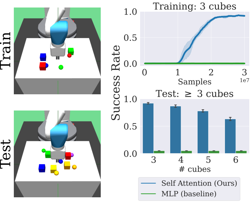
Figure 1:
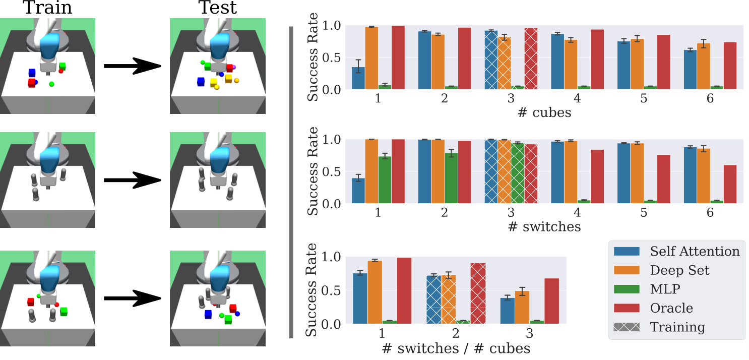
A family of tasks where the agent is trained to re-arrange three cubes (top-left), but tested zero-shot to re-arrange anywhere from three to six cubes (bottom-left). Reinforcement learning (RL) with standard MLPs fails to even learn the 3-cube task. Our self-attention based policy can learn the three cube task, and also solve tasks with more cubes using no additional data.
2 Related Work
Unlike hierarchical methods that explicitly learn macro-actions, this approach changes policy architecture while retaining end-to-end low-level learning. Its attention operates over objects and goals, rather than trajectory history. It connects entity-centric control with permutation-invariant neural networks.
3 Problem Formulation and Architectures
The framework specifies entity-based tasks and compares three ways to represent their policies.
3.1 Problem Setup
An EFMDP contains an agent state, a set of entity states, and matching subgoals. Rewards aggregate entity-level outcomes; transitions and rewards are unchanged by consistently reordering entity–goal pairs. Entity identities can remain encoded in their features.
The symmetry makes optimal action values permutation-invariant and permits an invariant optimal policy. The source states the stronger claim that every optimal policy is invariant; when optimal actions tie, this requires a consistent invariant tie-breaking rule. The architecture motivation does not depend on that stronger wording.
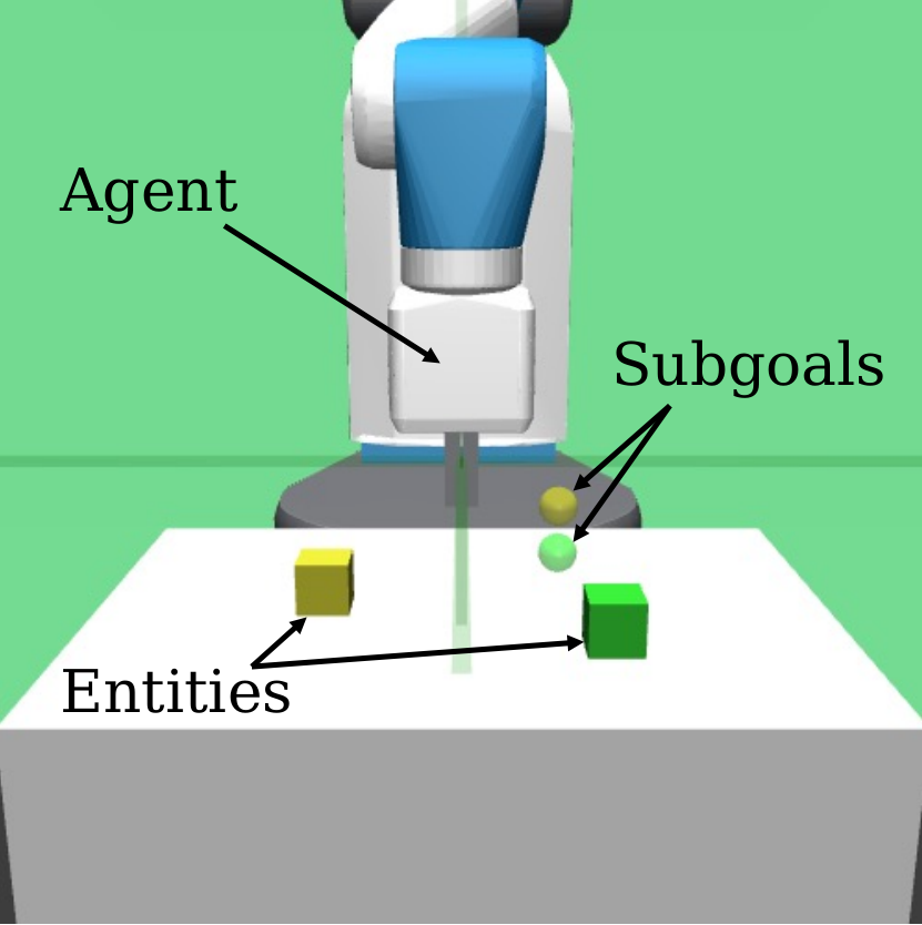
Figure 2: In an EFMDP, an agent interacts with entities that have corresponding subgoals. This framework can model rearrangement, strategic game playing, and multi-agent systems. In this “pushing and stacking” example, the agent must move the green cube to its subgoal (indicated by the green sphere), then stack the yellow cube on top of the green cube.Equations 1–5
(1)
(2)
(3)
(4)
(5)
Figure 3: Visualizations of implementing an entity-based goal conditioned policy using either Deep Sets (left) or Self Attention (right). The policy receives state containing agent state and entity states . The goal contains subgoals for each entity. Both policies arrange the input into vectors , one per entity. The Deep Set policy processes each independently with MLP , aggregates the outputs, and maps the result to an action using MLP . The self attention encoder produces output and uses self-attention (Eq. 11) to model interactions between the entities/subgoals. The are mapped to an action by summation and an MLP .
An MLP concatenates all states and goals into a fixed-size vector. Testing with more entities requires padding during training to reserve enough input slots; permutation invariance must be learned from data.
Equations 6–7
(6)
(7)
3.3 Deep Sets
Deep Sets applies a shared encoder to each entity, its subgoal, and the shared agent state, sums those features, then predicts an action. Pooling removes dependence on entity order and accepts variable set sizes. General approximation properties require sufficiently expressive component networks. [38]
Equations 8–10
(8)
(9)
(10)
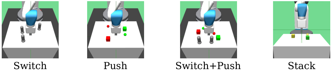
Figure 4: Illustrations of the robot manipulation environments we study. They consist of subtasks such as pushing a cube to its (spherical) target, flipping a switch to a specified position, and stacking one cube on top of another. The overall task can involve multiple entities and subtasks as well as their combinations (pushing cubes and flipping switches).
3.4 Self Attention
Self attention exchanges information among entity–goal representations before summing them into an action. The encoder omits positional encodings and causal masks so arbitrary input order has no effect. Compared with independent entity encoding, it provides a stronger bias for interactions among objects. [36]
Equation 11
(11)
4 Experiments and Evaluation
Evaluation separates training efficiency, zero-shot transfer to different entity counts, and combining previously learned subtasks without new training.
Environment Description
A simulated Fetch robot pushes cubes, flips switches, and stacks blocks. Task families vary object counts and combinations. A hand-designed oracle sequentially invokes single-subtask policies; it can fail because it does not account for interactions, so it is not a guaranteed-success upper bound.
4.1 Efficiency of Learning
Success requires every subgoal. Reinforcement learning uses DDPG with HER, applying the chosen architecture to both actor and critic. Imitation learning fits actions from successful trajectories generated by trained agents. Curves report five seeds with 95% confidence intervals.
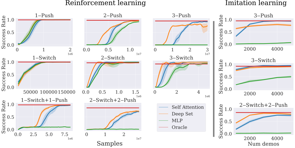
Figure 5:
Training on environments of varying complexity using either reinforcement or imitation learning. Each row corresponds to a single environment family (N-Push, N-Switch, and N-Switch + N-Push), where environments with larger contain more entities and are more complex. For RL (left), each plot is a training curve of success rate vs the number of steps taken in the environment. RL with standard MLPs can solve the simpler tasks such as 1-Push, but Deep Set and Self Attention policies are superior on the more complex environments. For IL (right), we show success rates of behavior cloning against number of expert demonstrations in the dataset. Both Deep Set and Self Attention policies far outperform the MLP even when given less data. Shaded regions indicate CIs over seeds.
All architectures learn simple single-entity tasks. Deep Sets and self attention learn substantially better as entity counts or mixed subtasks grow; the MLP often fails on harder tasks. Deep Sets commonly learns faster than attention, although their eventual performance is often similar.
The entity-based models also use demonstrations more effectively. In the reported three-cube pushing comparison with 5,000 demonstrations, self attention approaches full success while the MLP remains near zero.
Conclusions
The results favor explicit entity structure over a flat representation. Attention is especially useful on some interaction-heavy tasks, while the simpler Deep Sets design often has better sample efficiency. Neither architecture dominates every comparison.
Figure 6: Extrapolation capabilities of RL-trained policies with different architectures. Each row is an environment family that contains environments with a varying number of entities. Policies are trained on a single environment from each family before being tested on all the others, with no additional training. Bar charts show success rates in each environment, with the hatched bars corresponding to training environments. The Self Attention and Deep Set policies extrapolate beyond the training environment to solve tasks with more or fewer entities than seen in training, while MLP policies struggle on more complex testing environments. Error bars are CIs on 5 seeds.
4.2 Zero-Shot Extrapolation Capabilities
Policies trained on three cubes or switches are tested with one through six; mixed policies train with two of each and test with one through three. Checkpoints are selected by performance on training tasks. Structured policies often extrapolate well, but attention can fail on single-entity cases after multi-entity training. Deep Sets generalizes better in many of these tests.
4.3 Zero-Shot Stitching to solve novel tasks
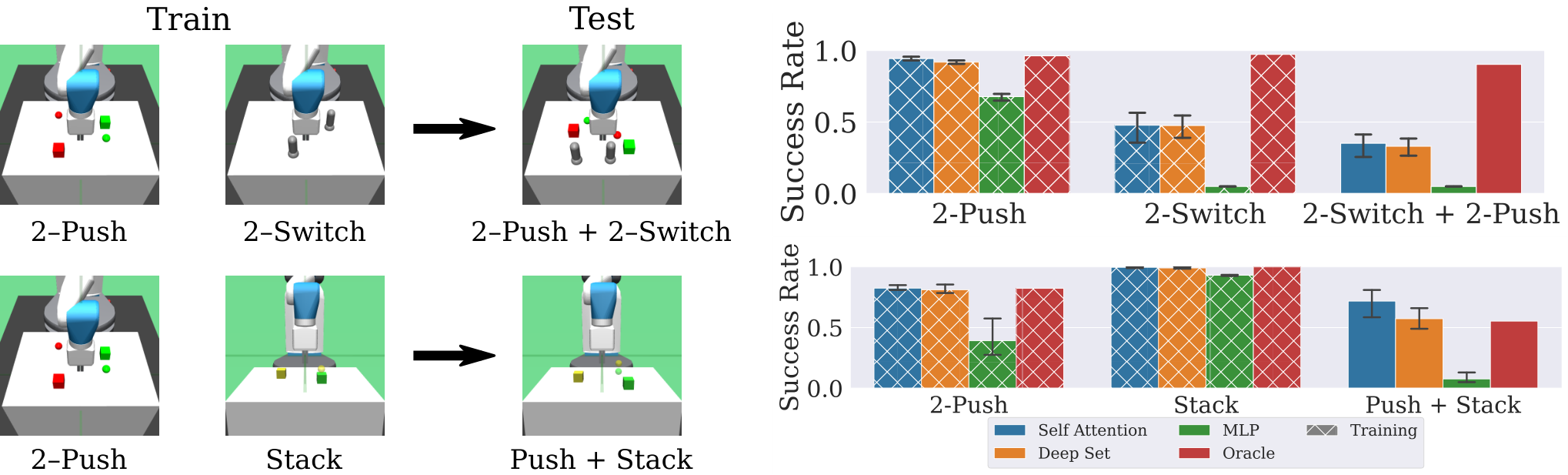
A single policy trains on separate task families and is then tested on their combination. Attention achieves about 60% success on pushing followed by stacking, versus roughly 5% for an MLP, despite never training on that combination. Mixed switch-and-push performance remains limited partly because joint training itself is difficult; learned composition is useful but incomplete.
Figure 7: Left: each row corresponds to a setting where policies are evaluated on test tasks that require stitching together skills learned in training, with no additional data. In the top setting, a single agent is trained on 2-Switch and 2-Push, and must solve 2-Switch+2-Push at test time. In the bottom setting, a single agent is trained on 2-Push and Stack, and must solve Push + Stack at test time. Right: average success rates of policies with different architectures in each setting. Deep Set and Self Attention policies are moderate successful at solving the test tasks, and are comparable to the Oracle in Push + Stack. The MLP fails to achieve nontrivial success rates on both test environments. Error bars indicate CIs over seeds.
5 Conclusion
Architectural symmetry improves sample efficiency and selected forms of compositional generalization without handcrafted action primitives. The experiments assume structured state and goal vectors; discovering equivalent entities directly from images is left for future work.
Acknowledgements
The authors acknowledge colleagues who provided feedback, mentoring, and code review.
Appendix A Permutation invariance
The proof initializes value iteration with an invariant value function and shows each Bellman update preserves the symmetry by reindexing successor states. It assumes discrete state components for simplicity. Invariant optimal action values imply invariant sets of maximizing actions; a consistently chosen maximizer gives an invariant optimal policy.
Equations 12–17
(12)
(13)
(14)
(15)
(16)
(17)
Appendix B Environments
Actions command three end-effector displacements and one gripper coordinate; the latter is disabled when stacking is unnecessary. Episode length adds twenty steps per switch and fifty per cube subtask. States provide object pose, velocity, type, and robot information.
Most non-stacking experiments disable cube–cube collisions, although the gripper can still disturb other objects. Dense rewards reflect average goal distance; sparse rewards require every subgoal within tolerance. A supplementary experiment restores collisions.
Appendix C Training details
Training details specify algorithms, network sizes, optimization, and computational costs.
C.1 Reinforcement learning
DDPG gathers experience from sixteen parallel environments into one replay buffer, with two episodes per five gradient updates and HER on 80% of sampled minibatches. Shared discount is 0.98. Learning rates are 0.001 for MLP/Deep Sets and 0.0001 for attention.
Exploration and training duration vary by environment; fast and slow decay schedules are compared where indicated. Attention uses two four-head encoder blocks without dropout. Complete actor/critic specifications and schedules remain in the original tables.
Behavior-cloning datasets contain 1,000–5,000 generated trajectories, filtered to successful episodes. Policies minimize action squared error for 60,000 Adam updates with batch size 128 and the same architecture-specific learning rates as reinforcement learning.
Equation
C.3 Training and inference speed
Deep Sets has parameter count independent of entity count and linear per-entity computation. Attention’s pairwise interactions require quadratic work and memory. Its GPU forward pass is slower, but total training times are similar in these small environments because simulation dominates; tests contain fewer than ten entities.
Figure 8: Left: the time (in milliseconds) it takes for each policy architecture to execute a single forward pass on a single input observation from the N-Push environments, where . The self attention policy is significantly slower, while the Deep Set and MLP policies are comparable. Right: Real world reinforcement learning times (in hours) training each policy/critic architecture on the N-Push environments. Although the Self Attention policy is slightly slower, all policies train at comparable speeds in the same environment. This suggests that environment simulation, not policy execution, is the dominant time consuming element.
Appendix D Further comparisons
Additional comparisons vary the Deep Sets output network and restore cube collisions.
D.1 Deep set architecture size
A two-layer output network improves some training and push-then-stack results, but extrapolates worse to five or six cubes than the one-layer version. Model capacity therefore trades off different forms of generalization rather than uniformly helping.
Figure 9: Comparison of N-Push extrapolation and Push + Stack stitching performance when using small and large variants of the Deep Set policy architecture. The small version implements with a 1-layer linear map, while the large version implements with a 2-layer MLP. For N-Push, the larger network achieves greater success rates in the training environment (3 cubes) but is actually worse when extrapolating to 5 or 6 cubes. On the other hand, the larger Deep Set displays superior stitching capability and achieves a higher average success rate when generalizing to Push + Stack from 2-Push and Stack.
D.2 N-Push with cube-cube collisions
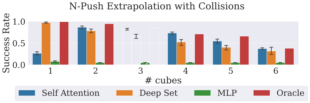
With cube–cube collisions enabled, success drops across methods by roughly the reported 15%, and attention often overtakes Deep Sets. These results support relational modeling when entities physically interact, while also showing the main collision-disabled setting is easier.
Figure 10: N-Push extrapolation with cube-cube collisions enabled. All methods observe some drop in performance relative to Figure 6, where N-Push has cube-cube collisions disabled. Self Attention tends to outperform Deep Sets when collisions enabled, likely because its relational inductive biases are better suited to handling interactions between entities that arise from collisions.
39 references
Andrychowicz et al. (2017)
Andrychowicz, M., Wolski, F., Ray, A., Schneider, J., Fong, R., Welinder, P.,
McGrew, B., Tobin, J., Abbeel, P., and Zaremba, W.
Hindsight experience replay.
arXiv preprint arXiv:1707.01495, 2017.
Bacon et al. (2017)
Bacon, P.-L., Harb, J., and Precup, D.
The option-critic architecture.
In Proceedings of the AAAI Conference on Artificial
Intelligence, volume 31, 2017.
Bapst et al. (2019)
Bapst, V., Sanchez-Gonzalez, A., Doersch, C., Stachenfeld, K., Kohli, P.,
Battaglia, P., and Hamrick, J.
Structured agents for physical construction.
In International Conference on Machine Learning, pp. 464–474. PMLR, 2019.
Batra et al. (2020)
Batra, D., Chang, A. X., Chernova, S., Davison, A. J., Deng, J., Koltun, V.,
Levine, S., Malik, J., Mordatch, I., Mottaghi, R., et al.
Rearrangement: A challenge for embodied ai.
arXiv preprint arXiv:2011.01975, 2020.
Bronstein et al. (2021)
Bronstein, M. M., Bruna, J., Cohen, T., and Veličković, P.
Geometric deep learning: Grids, groups, graphs, geodesics, and
gauges.
arXiv preprint arXiv:2104.13478, 2021.
Burgess et al. (2019)
Burgess, C. P., Matthey, L., Watters, N., Kabra, R., Higgins, I., Botvinick,
M., and Lerchner, A.
Monet: Unsupervised scene decomposition and representation.
arXiv preprint arXiv:1901.11390, 2019.
Carvalho et al. (2021)
Carvalho, W., Liang, A., Lee, K., Sohn, S., Lee, H., Lewis, R. L., and Singh,
S.
Roma: A relational, object-model learning agent for sample-efficient
reinforcement learning.
2021.
Chen et al. (2021)
Chen, L., Lu, K., Rajeswaran, A., Lee, K., Grover, A., Laskin, M., Abbeel, P.,
Srinivas, A., and Mordatch, I.
Decision transformer: Reinforcement learning via sequence modeling.
arXiv preprint arXiv:2106.01345, 2021.
Dietterich (2000)
Dietterich, T. G.
Hierarchical reinforcement learning with the maxq value function
decomposition.
Journal of artificial intelligence research, 13:227–303, 2000.
Haarnoja et al. (2018)
Haarnoja, T., Zhou, A., Abbeel, P., and Levine, S.
Soft actor-critic: Off-policy maximum entropy deep reinforcement
learning with a stochastic actor.
In International conference on machine learning, pp. 1861–1870. PMLR, 2018.
Huang et al. (2019)
Huang, D.-A., Nair, S., Xu, D., Zhu, Y., Garg, A., Fei-Fei, L., Savarese, S.,
and Niebles, J. C.
Neural task graphs: Generalizing to unseen tasks from a single video
demonstration.
In Proceedings of the IEEE/CVF Conference on Computer Vision
and Pattern Recognition, pp. 8565–8574, 2019.
Huang et al. (2017)
Huang, G., Liu, Z., Van Der Maaten, L., and Weinberger, K. Q.
Densely connected convolutional networks.
In Proceedings of the IEEE conference on computer vision and
pattern recognition, pp. 4700–4708, 2017.
Janner et al. (2021)
Janner, M., Li, Q., and Levine, S.
Offline reinforcement learning as one big sequence modeling problem.
Advances in Neural Information Processing Systems, 34, 2021.
Jiang et al. (2019)
Jiang, Y., Gu, S., Murphy, K., and Finn, C.
Language as an abstraction for hierarchical deep reinforcement
learning.
arXiv preprint arXiv:1906.07343, 2019.
Karch et al. (2020)
Karch, T., Colas, C., Teodorescu, L., Moulin-Frier, C., and Oudeyer, P.-Y.
Deep sets for generalization in rl.
arXiv preprint arXiv:2003.09443, 2020.
Li et al. (2020)
Li, R., Jabri, A., Darrell, T., and Agrawal, P.
Towards practical multi-object manipulation using relational
reinforcement learning.
In 2020 IEEE International Conference on Robotics and
Automation (ICRA), pp. 4051–4058. IEEE, 2020.
Lillicrap et al. (2015)
Lillicrap, T. P., Hunt, J. J., Pritzel, A., Heess, N., Erez, T., Tassa, Y.,
Silver, D., and Wierstra, D.
Continuous control with deep reinforcement learning.
arXiv preprint arXiv:1509.02971, 2015.
Lin et al. (2022)
Lin, Y., Wang, A. S., Undersander, E., and Rai, A.
Efficient and interpretable robot manipulation with graph neural
networks.
IEEE Robotics and Automation Letters, 2022.
Locatello et al. (2020)
Locatello, F., Weissenborn, D., Unterthiner, T., Mahendran, A., Heigold, G.,
Uszkoreit, J., Dosovitskiy, A., and Kipf, T.
Object-centric learning with slot attention.
arXiv preprint arXiv:2006.15055, 2020.
Nanbo et al. (2020)
Nanbo, L., Eastwood, C., and Fisher, R. B.
Learning object-centric representations of multi-object scenes from
multiple views.
In 34th Conference on Neural Information Processing Systems,
2020.
Parr & Russell (1998)
Parr, R. and Russell, S.
Reinforcement learning with hierarchies of machines.
Advances in neural information processing systems, pp. 1043–1049, 1998.
Schaul et al. (2015)
Schaul, T., Horgan, D., Gregor, K., and Silver, D.
Universal value function approximators.
In International conference on machine learning, pp. 1312–1320. PMLR, 2015.
Sinha et al. (2020)
Sinha, S., Bharadhwaj, H., Srinivas, A., and Garg, A.
D2rl: Deep dense architectures in reinforcement learning.
arXiv preprint arXiv:2010.09163, 2020.
Tang & Ha (2021)
Tang, Y. and Ha, D.
The sensory neuron as a transformer: Permutation-invariant neural
networks for reinforcement learning.
Advances in Neural Information Processing Systems, 34, 2021.
Vaswani et al. (2017)
Vaswani, A., Shazeer, N., Parmar, N., Uszkoreit, J., Jones, L., Gomez, A. N.,
Kaiser, Ł., and Polosukhin, I.
Attention is all you need.
In Advances in neural information processing systems, pp. 5998–6008, 2017.
Veerapaneni et al. (2020)
Veerapaneni, R., Co-Reyes, J. D., Chang, M., Janner, M., Finn, C., Wu, J.,
Tenenbaum, J., and Levine, S.
Entity abstraction in visual model-based reinforcement learning.
In Conference on Robot Learning, pp. 1439–1456. PMLR, 2020.
Zaheer et al. (2017)
Zaheer, M., Kottur, S., Ravanbakhsh, S., Poczos, B., Salakhutdinov, R., and
Smola, A.
Deep sets.
arXiv preprint arXiv:1703.06114, 2017.
Zambaldi et al. (2018)
Zambaldi, V., Raposo, D., Santoro, A., Bapst, V., Li, Y., Babuschkin, I.,
Tuyls, K., Reichert, D., Lillicrap, T., Lockhart, E., et al.
Relational deep reinforcement learning.
arXiv preprint arXiv:1806.01830, 2018.