Overview
The supplementary material defines the two supplied domain-specific languages, their differentiable executors, candidate lexical templates, an expected-execution example and proof, and the exact benchmark splits. These details expose substantial structural assumptions behind the strong generalization results.
At a glance
Grammar-Based Grounded Lexicon Learning associates each word with a syntactic type, semantic program, and optional grounded concept embedding. A small combinatory grammar composes these entries into executable sentence meanings. Joint chart parsing and local expected execution reduce the candidate search space. The experiments show strong generalization on filtered synthetic visual questions and generated action-language tasks, under fixed languages, limited candidate programs, and context-independent lexical meanings.
1 Introduction
The lexicalist hypothesis places most learned linguistic information in word entries while keeping composition rules small and fixed. G2L2 jointly learns entries and concept embeddings from grounded supervision, such as image–question–answer triples. It extends neuro-symbolic concept learning with a grammar-based parser. Avoiding annotated lexicons or question programs does not mean learning all structure: the domain-specific language, combinatory rules, candidate templates, object proposals, and training curriculum are supplied.
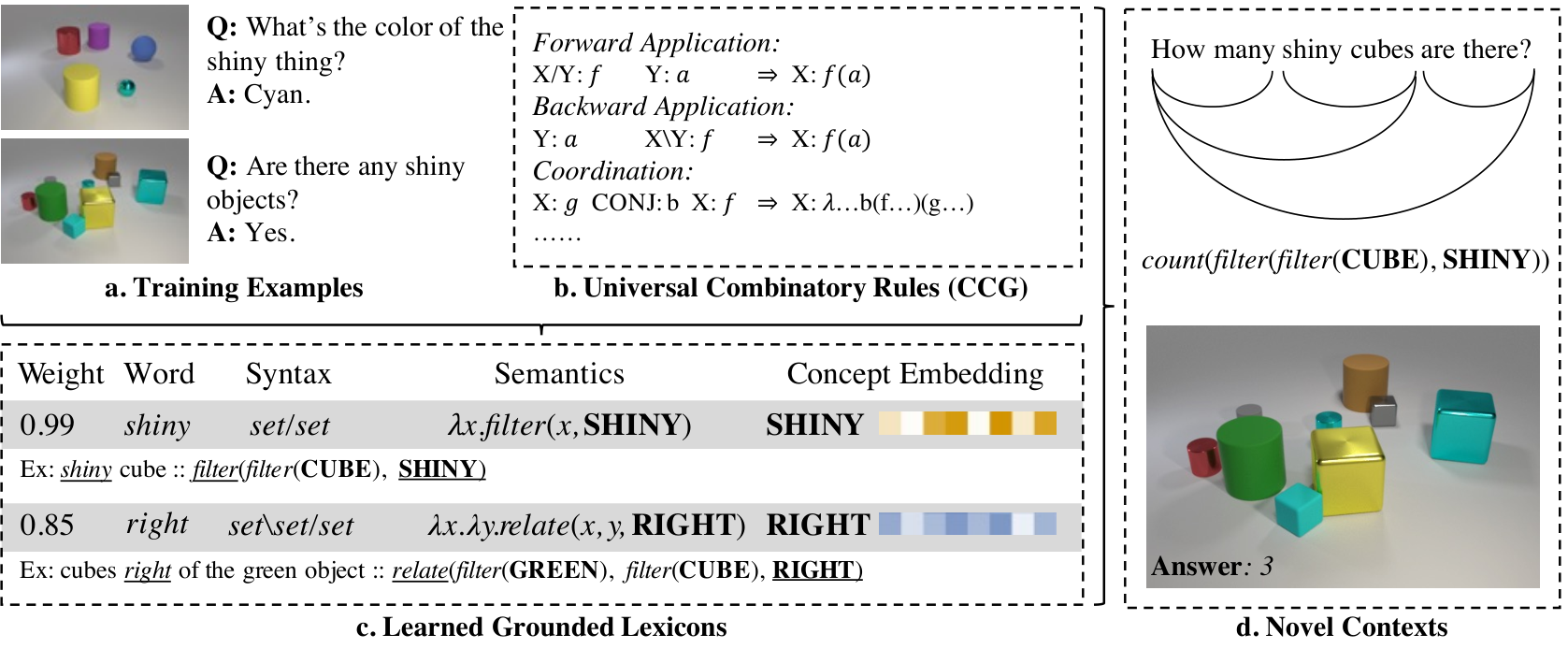
2 Grammar-Based Grounded Lexicon Learning
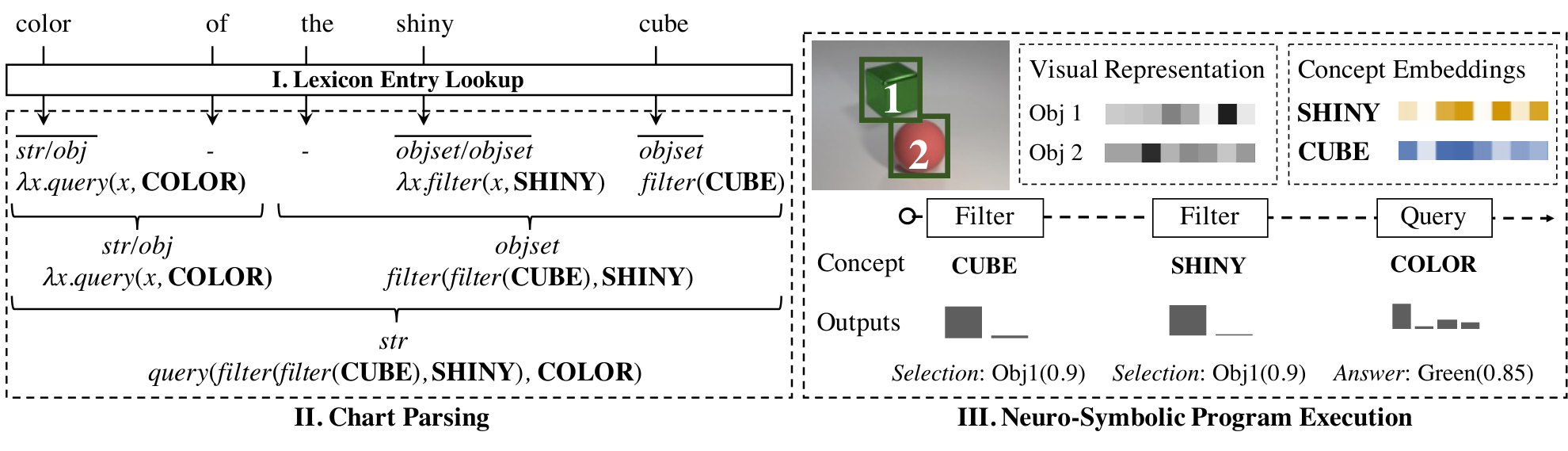
For each token, the model retrieves candidate lexical entries. Chart parsing combines compatible syntactic types and their programs, and a differentiable executor evaluates grounded meanings. Answer error trains lexical weights and perceptual concept embeddings. The demonstrated implementation assumes one context-independent entry per word type and uses empty entries for words the supplied language cannot represent.
2.1 Grounded Lexicon
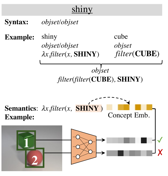
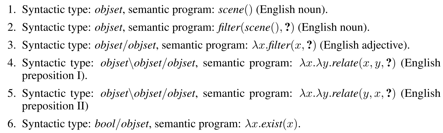
Primitive syntactic types correspond to domain values; directional functor types specify an argument’s type and whether it occurs to the left or right. The semantic entry is a typed program with learnable concept embeddings. Candidate programs are bounded in arity and depth, then expanded over allowed argument orders and assigned scalar weights.
Although the formalism can store multiple entries, the experiments assume no lexical ambiguity and aim to select one entry per word. Visual reasoning uses a small hand-selected template set; navigation enumerates a larger but still restricted set. These assumptions simplify learning and exclude many ordinary linguistic phenomena.
2.2 Program Execution
The executor represents object sets as soft masks over detected objects. A filter compares object and concept embeddings and multiplies the resulting scores by the incoming mask. Subsequent operations compose these values to answer a query. The appendix changes the original NS-CL minimum/maximum set operators to product-based operations to support expectation calculations. Soft values are used computationally; calibration is not evaluated.
2.3 Joint Chart Parsing and Expected Execution (CKY-E2)
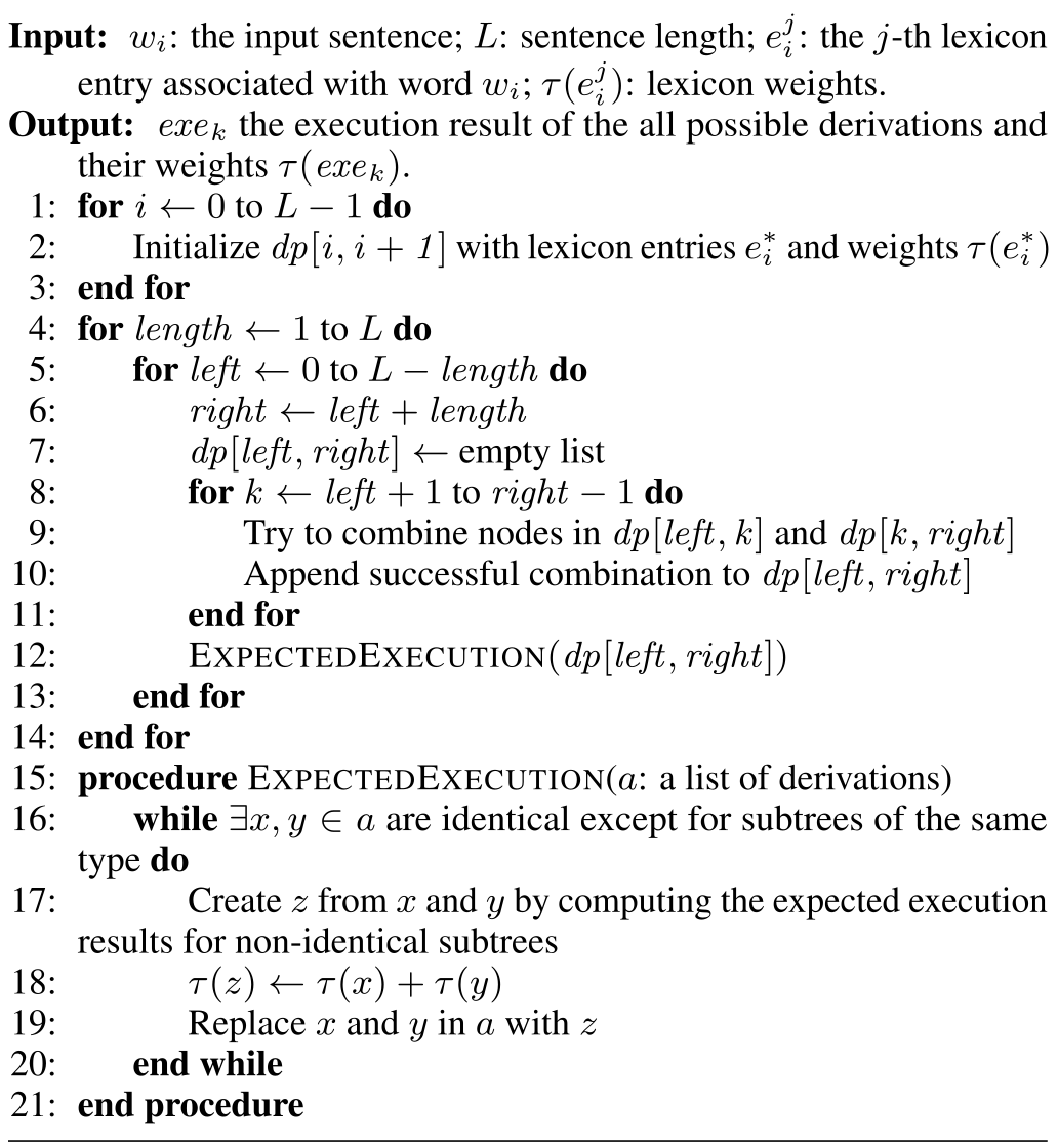
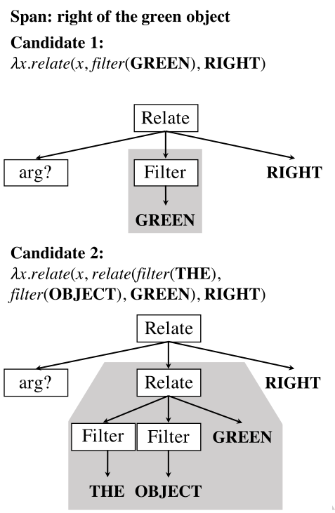
CKY-E2 extends chart parsing by merging derivations that share a program structure except for grounded subtrees of the same type. Those subtrees are replaced by a weighted mean of their execution values. This avoids enumerating every complete lexical combination. Exactness requires each subsequent composition to commute with the relevant expectation, including independence assumptions for products; nonlinear quantifiers or minimum/maximum operations generally make the procedure approximate.
The stated O(L³M) cost relies on bounded arity and a restricted number of residual program layouts. Appendix B proves a limited per-span representation bound, not an unrestricted grammar theorem. There is also a source notation inconsistency: Algorithm 1 and the main merge example add log weights, whereas Appendix A uses log-sum-exp to combine alternative derivations. The original formulas are preserved, and the appendix convention is the normalized-mixture interpretation.
Equations
2.4 Learning
The written objective is the probability-weighted loss over complete derivations, optimized through lexical weights and concept modules. The expected-execution proof concerns the mean execution result. For a nonlinear loss, loss of that mean is generally different from the expected loss; preserving the mean alone therefore does not establish exact computation of every stated training objective. The paper does not fully resolve that distinction, and the edition retains both the objective and its qualified inference claims.
Equation
3 Experiment
Two controlled domains test data efficiency and compositional transfer: a regenerated subset of CLEVR visual questions and SCAN instruction-to-action sequences. Reported successes should be read alongside dataset filtering, manually supplied operation languages, and selection of successful SCAN training runs.
3.1 Visual Reasoning
CLEVR retains 208 of 425 templates, excluding coreference, same-related questions, and number comparisons. A length-based curriculum expands from short questions toward twenty-word questions. Ten percent of the training set is held out for development, and the original validation split supplies evaluation images/questions. Compared methods differ in program and concept supervision; G2L2 also depends on pretrained object detection.
Accuracy is 98.11% with 10% training data and 98.25% with the full set. On held-out compositions, it reaches 97.82% for purple, 98.59% for right, and 96.76% for count; on two-hop depth transfer it reaches 98.49%. The strongest margins are count and depth, whose best listed alternatives are 81.81% and 81.60%. G2L2 does not lead every standard, purple, or right column, despite broader claims in parts of the prose.
| Model | Prog? | Concept? | Standard | Compositional Generalization | Depth | |||||
| 10% | 100% | purple | right of | count | ||||||
| MAC [21] | N/N | N/N | 85.39 | 98.61 | 97.14 | 90.85 | 54.87 | 77.40 | ||
| TbD-Net [31] | Y/Y | N/N | 44.52 | 98.04 | 89.57 | 49.92 | 63.37 | 53.13 | ||
| NS-VQA [46] | Y/Y | Y/Y | 98.57 | 98.57 | 95.52 | 99.80 | 81.81 | 50.45 | ||
| NS-CL [30] | Y/N | Y/N | 98.51 | 98.91 | 98.02 | 99.01 | 18.88 | 81.60 | ||
| G2L2 (ours) | Y/N | Y/N | 98.11 | 98.25 | 97.82 | 98.59 | 96.76 | 98.49 | ||
3.2 Language-driven Navigation
SCAN maps generated instructions to sequences over six actions. The supplied string language constructs, concatenates, and repeats action sequences. Candidate meanings have at most two arguments and three operations, with restricted functor arguments and two syntactic categories; each word receives 178 candidates. Tests hold out jump compositions, around-right phrases, or longer output sequences.
Selected G2L2 runs score 100% on all reported splits, including output lengths up to forty-eight after training on at most twenty-two. This is not the success rate of an arbitrary training run: only 74 of one hundred runs reach perfect training accuracy; the rest average 94%. Runs failing that criterion are restarted, and the table averages ten valid runs. A common failure confuses the syntactic types of and/after, introducing attachment ambiguity. The benchmark is action-sequence translation, not physical navigation by a robot.
| Model | Simple | Compositional Generalization | Length | |||
| 10% | 100% | jump | around right | |||
| seq2seq [40] | 0.93 | 0.99 | 0.00† | 0.00† | 0.15 | |
| Transformer [44] | 0.71 | 0.78 | 0.00 | 0.10 | 0.02 | |
| GECA [3] | 0.99 | 0.98 | 0.87† | 0.82† | 0.15 | |
| WordDrop [17]∗ | 0.56 | 0.62 | 0.52 | 0.70 | 0.18 | |
| SwitchOut [45]∗ | 0.99 | 0.99 | 0.98 | 0.97 | 0.17 | |
| SeqMix [17]∗ | – | – | 0.98‡ | 0.89‡ | – | |
| recomb-2 [2] | – | – | 0.88† | 0.82† | – | |
| G2L2 (ours) | 1.00 | 1.00 | 1.00 | 1.00 | 1.00 | |
4 Related Work
Lexicalist theories motivate separating rich word knowledge from a small rule inventory. The method differs from latent-tree neural models by storing typed semantic programs and compressed execution values at spans, and from conventional neural semantic parsers by explicitly constraining lexical composition. Compared with data augmentation, it supplies grammatical and semantic structure directly. Its claims concern these controlled inductive biases rather than a demonstration that unrestricted natural language has a unique context-independent lexicon.
5 Conclusion and Discussion
The framework supports interpretable lexical entries and strong constituent-level generalization in the evaluated settings. Open limitations include polysemy, context-dependent meaning, pragmatics, richer semantic languages, and reliable optimization. The broader-impact discussion identifies possible language-grounding biases and treats interpretability as a tool for examining them, without demonstrating their elimination. The acknowledgements credit identification and correction of a mathematical error; the remaining main-text/appendix notation discrepancies are retained and identified in the relevant notes.
Appendix A Domain Specific Languages and Neuro-Symbolic Reasoning
Both domains use manually designed types and deterministic tensor operations. Differentiability lets answer supervision train concept embeddings and lexical weights, but it does not remove the supplied semantic language or its restrictions. The appendix specifies which value types are actually merged by expected execution.
A.1 Visual Reasoning DSL
The visual language has six types and eight primitive operations. It removes unique because its context-dependent uses violate the one-entry-per-word assumption; relevant operations instead handle uniqueness internally. Tables 3 and 4 preserve the type representations and operation signatures, including source omissions and wording. This is a restricted CLEVR language rather than the full original question set.
| Type | Note | Representation |
| ObjConcept | Object-level concepts. | An embedding vector. |
| Attribute | Object-level attributes. | A vector of length , where is the number of |
| RelConcept | Relational concepts. | An embedding vector. |
| ObjectSet | A set of objects in the scene. | A vector of length , where is the number of objects in the scene. Each entry is a real value in , which can be interpreted as the probability that object is in this set. |
| Integer | An integer. | A single non-negative real value, which can be interpreted as the “expected” value of this integer. |
| Bool | A Boolean value. | A single real value in , which can be interpreted as the probability that this Boolean value is true. |
| Signature | Note |
| scene() ObjectSet | Return all objects in the scene. |
| filter(: ObjectSet, : ObjConcept) ObjectSet | Filter out a set of objects having the object-level concept (e.g., red) from the input object set. |
| relate(: ObjectSet, : ObjectSet, : RelConcept) ObjectSet | Filter out a set of objects in set that have the relational concept (e.g., left) with the input object . |
| intersection(: ObjectSet, : ObjectSet) ObjectSet | Return the intersection of set and set . |
| union(: ObjectSet, : ObjectSet) ObjectSet | Return the union of set and set . |
| query(: ObjectSet, : Attribute) ObjConcept | Query the attribute (e.g., color) of the input object . |
| exist(: ObjectSet) Bool | Check if the set is empty. |
| count(: ObjectSet) Integer | Count the number of objects in the input set. |
Object-centric scene representation.
A pretrained Mask R-CNN produces object boxes. ResNet-34 extracts region features using region-of-interest alignment and global image features; their concatenation represents each object. Thus the system learns grounded attribute representations while relying on an already trained mechanism for finding objects.
Neuro-symbolic realization.
Filtering multiplies the incoming mask by a sigmoid of the object–concept inner product. Intersection uses elementwise multiplication, and union uses one minus the product of complements. These product-logic choices replace NS-CL’s minimum and maximum to make the chosen expectation operations tractable. Exactness for multiplied uncertain inputs still requires the factorization conditions stated in the formal analysis.
Equation
Example.
The shiny-cubes example starts with three selected objects, applies cube scores and then shiny scores, and obtains a mask [0.08, 0.08, 0.81]. Summing gives the soft count 0.97. Table 5 retains every step; the example illustrates differentiable computation rather than exact Boolean set membership.
| Program | Type | Value | ||||
| ObjectSet | ||||||
| ObjectSet | ||||||
|
|
|
| ||||
| Integer |
Expected execution.
Only object-set subprograms are merged in the visual implementation. Their output vectors are averaged using softmax-normalized derivation weights, and the combined log weight is log-sum-exp of the alternatives. Integer and Boolean results could also be averaged, but occur only at sentence level here. This appendix rule differs from the simple weight addition printed in the main merge example and Algorithm 1.
Equation
Candidate lexicons.
The visual search uses ten listed templates: scene or filtered nouns, adjective filtering, two relation orientations, existence, counting, attribute query, generalized conjunction, and a specialized disjunction. Each word gets object-concept, relation-concept, and attribute representations as required by its candidates. Empty entries absorb unsupported words.
Generalized conjunction combines matching types, whereas disjunction uses an explicitly ad hoc type/rule because the set-theoretic language cannot express all ordinary word meanings. Table 6 shows a learned example with empty entries for are and there. These implementation choices materially restrict the claimed automatic discovery of lexical semantics.
Equations

| Word Type | Syntactic Type | Semantic Program |
| are | <EMPTY> | <EMPTY> |
| there | <EMPTY> | <EMPTY> |
| any | ||
| shiny | ||
| cubes | objset |
A.2 Language-Driven Navigation DSL
The navigation language has action-sequence and integer types and supports empty strings, primitive actions, integer constants, concatenation, and repetition. Integers are restricted to two, three, and four. Table 7 retains all operations. The output is a symbolic action string rather than a trajectory governed by a physical environment.
| Signature | Note |
| empty() ActSeq | Create an empty string (of length 0). |
| newprim() ActSeq | Create a string containing only one primitive action. In SCAN, there are in total 6 primitives. |
| newint() Integer | Create a single integer. In SCAN, we only support integers {2, 3, 4}. |
| concat(: ActSeq, : ActSeq) ActSeq | Concatenate two input strings. |
| repeat(: ActSeq, : Integer) ActSeq | Repeat the input string for multiple times. |
Probabilistic string representation.
A probabilistic string stores a categorical length distribution and conditional token distributions indexed by length, position, and action. Concatenation sums over possible length partitions; repetition maps lengths and positions to the repeated source. This finite tensor representation is bounded by a maximum sequence length and vocabulary. The original equations are retained; the repetition equation’s conditional-token row uses an L symbol where the surrounding representation uses C, a source notation inconsistency.
Equations
Expected execution.
Expected execution merges action-sequence values by averaging length probabilities and weighting conditional token distributions by both derivation and length probability. It retains these marginals, rather than the complete distribution over symbolic programs or every dependency among sequence tokens. The invariance claim remains conditional on the supported operations and factorization assumptions.
Equation
Candidate lexicons.
Enumeration permits at most three operations, two arguments, one functor-typed argument, and no integer argument. Only six listed syntactic forms are allowed after splitting action-sequence meanings into S and V categories. This produces 178 candidates per word. Table 8 retains the examples, including higher-order functions; the candidate set is far narrower than arbitrary programs of the domain.
| Type | Program (Note) | ||||||
|
| ||||||
|
| ||||||
|
| ||||||
|
| ||||||
|
|
Appendix B Delve Into Expected Execution
The appendix explains local expectation merging with an arithmetic example, then states its invariance condition, restricted complexity argument, and relationship to grammar-based inference. The analysis establishes preservation of a mean under specified operations, not preservation of the full distribution or every nonlinear training loss.
B.1 CKY-E2 In An Arithmetic Domain
Three toy tokens have four equally weighted derivations producing three, four, six, and nine, with mean 5.5. Merging the first constituent produces mean 2.5; the remaining alternatives produce 3.5 and 7.5, again averaging 5.5. Tables 9 and 10 and the display retain the complete example. Addition and multiplication by fixed constants preserve this mean; the example does not show that the four derivations or their squared losses are identical after merging.
Equation
| Word Type | Syntactic Type | Semantic Program | (Weight) |
| ONE | N | 1 | 1.0 |
| PLUS_ONE | N\N | 0.5 | |
| PLUS_ONE | N\N | 0.5 | |
| MUL_THREE | N\N | 0.5 | |
| MUL_THREE | N\N | 0.5 |
|
|
|
|
| |||||||
| 1 | N | ||||||||||
| 2 | N | ||||||||||
| 3 | N | ||||||||||
| 4 | N |
B.2 Formal Properties of CKY-E2
The proof factors derivation weights over two constituents and assumes a composition function whose expectation equals composition of the input expectations. Under those assumptions, local merging can be repeated over a derivation tree. The subsequent complexity argument uses a restricted inventory of primitive, unary, binary, and partly applied binary types.
Expectation invariance.
Normalize alternative weights separately for each constituent. If composition preserves expectation under that product distribution, summing all pairwise executions equals composing the two weighted mean executions. Affine operations and products of independent inputs can satisfy this; minima, maxima, and general nonlinear functions do not. Independence and the semantic operation’s algebra are part of the guarantee, not optional implementation details.
Equations
Complexity.
For one primitive type and the stated unary/binary entry forms, a span stores at most one merged primitive value, N₁ unary entries, N₂ binary entries, and N₂ partially applied entries. Across quadratically many spans this yields polynomial storage and a tractable restricted parser. The main O(L³M) claim assumes fixed bounded structure; the appendix does not prove that every richer grammar or program language has the same bound.
B.3 Connection with Other Parsing Models
The parser can be interpreted as jointly constructing syntax trees and meaning programs. Expected execution compresses the latter based on grounded values. This viewpoint clarifies both its relationship to synchronous grammars and what information is discarded by storing means.
Connection with synchronous grammars.
A synchronous grammar relates a linguistic derivation to a semantic program, but here the program is learned through distant grounded supervision rather than directly paired program annotations. Local expected execution compresses possible meanings after grounding a span.
Connection with sum-product CKY.
Both methods exploit context-free structure, but ordinary sum-product chart parsing propagates weights over its represented alternatives, while CKY-E2 stores expected execution values. The paper argues that an explicit distribution over all programs is impractical in its setting. The advantage therefore depends on accepting the information discarded by moment-based compression and the operations under which that compression is valid.
Appendix C Experimental Setup And Analysis
The appendix defines the regenerated visual-question dataset and the official SCAN partitions, then diagnoses baseline errors. Exact splits and supplied supervision matter when interpreting compositional generalization. The two datasets are reported as BSD licensed.
C.1 Visual Reasoning: CLEVR
All visual splits start from regenerated questions using the selected unambiguous templates. The analysis distinguishes failures of a semantic parser from failures of its execution modules, since correct answers can sometimes result from an incorrect program.
Baselines.
MAC reasons through attention. TbD-Net and NS-VQA use a supervised sequence-to-sequence parser; NS-CL uses a jointly trained sequence-to-tree parser with additional concept-token embeddings. The latter still receives a concept vocabulary. These representation and supervision differences prevent treating the comparison as a change only to the parsing algorithm.
Dataset generation.
The authors retain 208 of 425 CLEVR templates, manually excluding coreference, same-related questions, and number comparisons. They regenerate questions to match the original question count. This removes cases that violate the assumption of one lexical entry per word; the evaluated dataset is not the full original CLEVR distribution.
Split: data efficiency.
The 10%-data split evaluates on the same standard test distribution. Program-based baseline parsers are almost perfect, so remaining differences primarily reflect their perceptual/execution modules. NS-VQA’s object recognizer is already trained with direct object-level labels, an important qualification to its apparent data efficiency.
Split: compositional generalization (purple).
For purple, training retains questions without that word or with length at most seven including punctuation; testing uses longer purple questions. Baseline parsers are nearly perfect, making grounding and module composition the main sources of error. The main text’s six-word cutoff and this seven-token threshold use different counting conventions, explicitly including punctuation here.
Split: compositional generalization (right).
For right, training retains questions without the word or with at most twelve tokens; testing uses longer matching questions. NS-CL parsing is nearly perfect, while the shared TbD-Net/NS-VQA parser is about 91% accurate. The authors hypothesize that TbD-Net’s deeper relational module is harder to train. G2L2’s score is strong but lower than NS-VQA’s listed right-split accuracy.
Split: compositional generalization (count).
For count, training permits counting questions of at most nine tokens and otherwise noncounting questions. Testing combines counting with longer structures whose constituents appeared separately in training. The shared sequence parser reaches 70.8% program accuracy; NS-CL sometimes selects the wrong final object filter. G2L2’s explicit lexical composition improves this test, but the result remains within the supplied candidate language.
Split: depth generalization.
Depth transfer trains on zero- and one-hop questions and tests two-hop references. The shared sequence parser reaches only 1.7% program accuracy and sometimes generates invalid programs. NS-CL maintains syntactic program validity but can omit needed operations. Question-answer accuracy may overstate program correctness when an erroneous program happens to return the right answer; G2L2 reaches 98.49% answer accuracy here.
C.2 Language-Driven Navigation: SCAN
SCAN evaluation uses exact output-sequence matching. The splits isolate sparse primitive exposure, unseen phrase combinations, and output-length extrapolation. All language comes from a finite generator, so these results do not directly measure unrestricted instruction understanding.
Split: data efficiency.
The official simple split uses eighty percent of generated pairs for training. The reduced-data experiment samples ten percent of that training set uniformly across input lengths. Both use the same simple test split; this is data efficiency within the generated distribution.
Split: compositional generalization (jump).
Jump appears only as an isolated training command, while test commands place it in composed structures such as repetition. The task tests whether the learned lexical type and action meaning can be reused with familiar constructions.
Split: compositional generalization (around right).
Training excludes every phrase containing around right; the held-out phrase is not itself a complete command. Test commands require combining meanings learned from phrases such as around left and opposite right. This differs from jump, which does receive an isolated example.
Split: length generalization.
Training outputs have at most twenty-two actions, while test outputs can reach forty-eight. Perfect selected-run performance therefore demonstrates sequence-length transfer within the supplied grammar and string operations, rather than arbitrary planning horizons.
Baseline models.
Most augmentation comparisons train sequence-to-sequence models on expanded datasets. GECA’s recombination rules can generate examples that also occur in the test set, particularly on compositional partitions; this is an explicit property of that baseline setup. Main-table values combine reproduced and cited results, and the G2L2 averages include only runs that attained perfect training accuracy.