At a glance
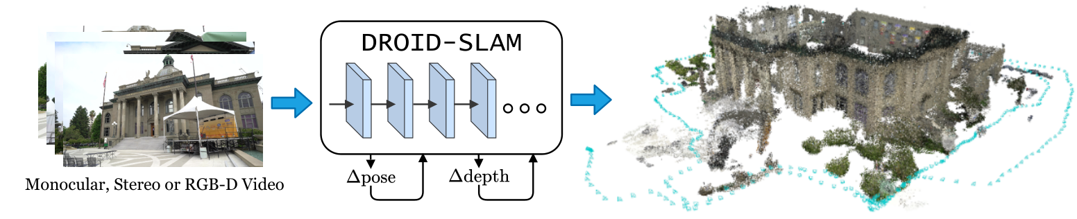
DROID-SLAM jointly refines camera poses and dense inverse-depth maps using learned correspondence updates and a differentiable bundle-adjustment layer. A model trained only on synthetic monocular clips can use monocular, stereo, or RGB-D video at inference. The reported benchmarks show fewer tracking failures and lower trajectory error, with substantial GPU and memory requirements. Code is available.
1 Introduction
The central idea is to let a network revise image correspondences while geometry determines the pose and depth updates. DROID extends RAFT’s recurrent refinement from a pair of flow fields to a graph of many frames, enabling loop closure and global optimization. Its DBA layer directly optimizes per-pixel depth, rather than coefficients of a learned depth basis. [49], [47], [48].
2 Related Work
Classical indirect methods minimize geometric reprojection error after feature detection; direct methods optimize image appearance. DROID uses dense learned image information with a geometric objective. Earlier learned systems often operate on short windows or constrained depth representations; DROID maintains a longer-lived frame graph and global optimization. [31], [32], [5], [15], [16], [61], [9], [1], [47].
3 Approach
Each retained image has a camera pose in SE(3) and an inverse-depth value per pixel. Edges connect frames with overlapping views. The system updates these unknowns repeatedly and adds long-range edges when it recognizes previously mapped regions.
3.1 Feature Extraction and Correlation
Separate feature and context encoders produce maps at one-eighth image resolution. For each graph edge, all-pairs feature similarities form a four-dimensional correlation volume. A four-level pyramid and differentiable local lookup provide matching evidence near the correspondence predicted by the current geometry. [49].
Equation 1
| (1) |
3.2 Update Operator
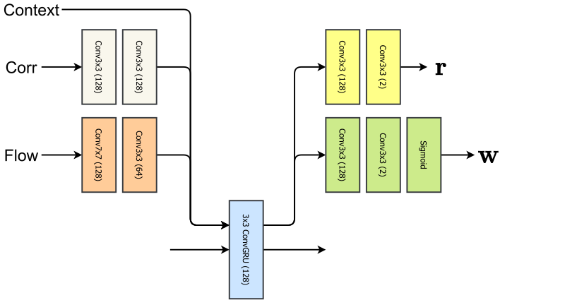
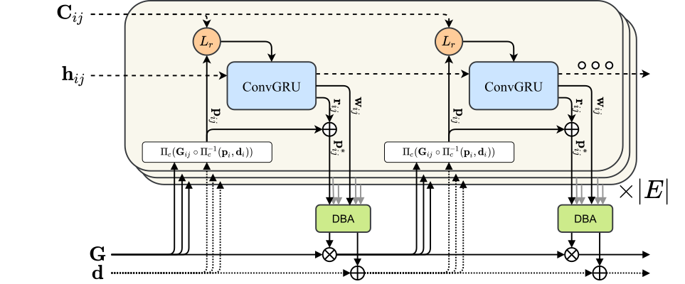
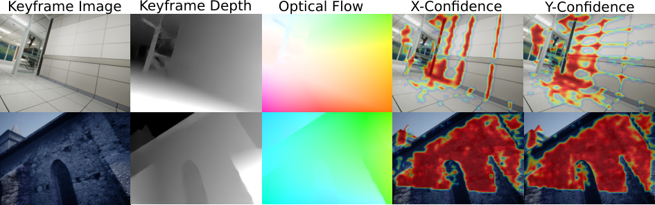
A convolutional GRU receives correlation lookups, induced optical flow, the preceding optimization residual, context features, and pooled global information. It predicts a correction to dense correspondences and confidence weights; additional pooled features predict positive depth damping and an upsampling mask.
DBA minimizes confidence-weighted geometric reprojection error against those corrected correspondences. A Gauss–Newton step jointly updates poses and inverse depths. The depth block is diagonal, so a Schur-complement solve eliminates it efficiently before recovering depth updates. Training differentiates through this optimization. Repeated updates are intended to converge to a consistent reconstruction; the paper does not prove global convergence.
Equations 2–5
| (2) |
| (3) |
| (4) |
| (5) |
3.3 Training
Training fixes the first two poses to ground truth to remove coordinate and scale ambiguity. Seven-frame clips are sampled with at least 50% overlap and approximately 8–96 pixels of adjacent flow. Pose and geometry-induced flow losses supervise every iteration, with later iterations weighted more heavily. LieTorch supports differentiation of rigid transforms. [50].
3.4 SLAM System
The front end selects keyframes, estimates incoming motion, and performs local bundle adjustment. The asynchronous back end rebuilds a co-visibility graph and refines all keyframes, including loop connections. Initialization gathers twelve sufficiently separated frames and runs ten updates. Non-keyframe poses are recovered with motion-only optimization; evaluation uses the complete trajectory.
Memory-efficient correlation lookup and a sparse CUDA implementation support large graphs. RGB-D adds a penalty toward measured inverse depth while allowing noisy or missing measurements to be refined. Stereo introduces a second camera and fixes the calibrated relative transform. Neither change requires retraining the correspondence network.
4 Experiments
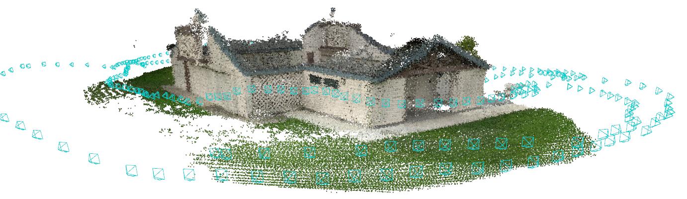
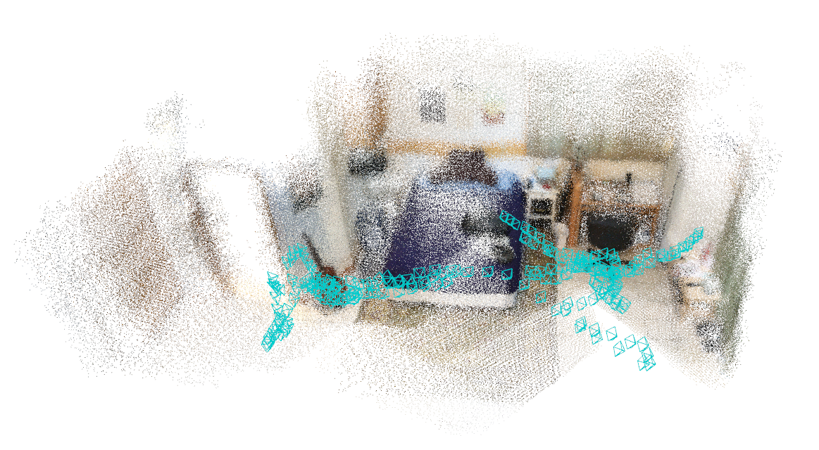
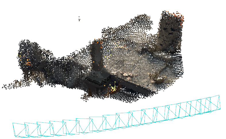
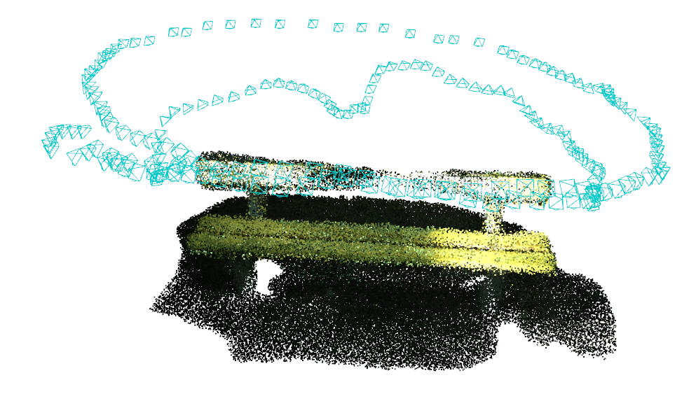
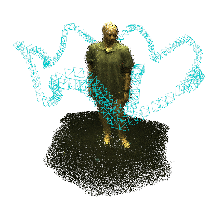
One model is trained on TartanAir monocular video for 250,000 steps using seven-frame clips and fifteen recurrent updates; training takes about one week on four RTX 3090 GPUs. Evaluation emphasizes trajectory accuracy and failure rate, rather than quantitatively testing dense map quality.
On the TartanAir competition metric, monocular and stereo error are 0.129 and 0.047, about 62% and 60% below the best listed competing submissions. The separate hard-sequence monocular table reports mean ATE of 0.24 m. These are different metrics and test summaries. [55], [54], [48].
On EuRoC monocular video, mean ATE is 0.022 m across eleven sequences. The reported 43% improvement over ORB-SLAM3 compares only the ten sequences that baseline completes; the larger 82% reduction uses methods with no failures. On the nine TUM freiburg1 sequences, DROID completes every run with mean ATE of 0.038 m. The table includes heterogeneous baselines: DeepTAM receives depth, and TartanVO uses ground truth to scale relative motion. [2], [5], [44], [60], [54].
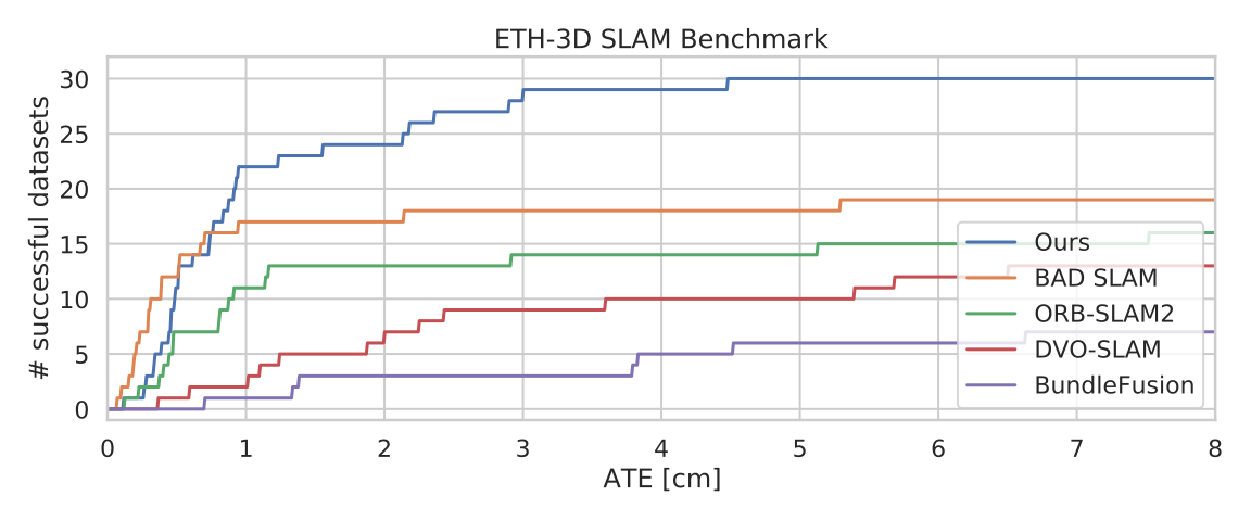
For RGB-D ETH3D, DROID successfully tracks 30 of 32 test sequences with image data and achieves test AUC of 207.79 versus 153.47 for BAD-SLAM. Completely dark sequences without image data are excluded. These rankings describe the paper’s evaluation, not a current leaderboard. [42].
Real-time experiments use two RTX 3090 GPUs, reduced resolution, and every-other-frame processing, averaging the incoming camera rates of 20 frames/s on EuRoC and 30 on TUM. TartanAir runs at 8 frames/s and is not real time. Some full-sequence evaluations require 24 GB of GPU memory; computational resources are the authors’ main stated limitation.
| Monocular | MH000 | MH001 | MH002 | MH003 | MH004 | MH005 | MH006 | MH007 | Avg |
|---|---|---|---|---|---|---|---|---|---|
| ORB-SLAM [31] | 1.30 | 0.04 | 2.37 | 2.45 | X | X | 21.47 | 2.73 | - |
| DeepV2D [48] | 6.15 | 2.12 | 4.54 | 3.89 | 2.71 | 11.55 | 5.53 | 3.76 | 5.03 |
| TartanVO [54] | 4.88 | 0.26 | 2.00 | 0.94 | 1.07 | 3.19 | 1.00 | 2.04 | 1.92 |
| Ours | 0.08 | 0.05 | 0.04 | 0.02 | 0.01 | 1.31 | 0.30 | 0.07 | 0.24 |
| Mono. | Stereo | |
|---|---|---|
| OV2SLAM [17] | 0.510 | 0.182 |
| VOLDOR [28] + COLMAP [41] | 0.440 | 0.177 |
| SuperGlue [39] + SuperPoint [13] + COLMAP [41] | 0.340 | 0.119 |
| Ours | 0.129 | 0.047 |
| MH01 | MH02 | MH03 | MH04 | MH05 | V101 | V102 | V103 | V201 | V202 | V203 | Avg | ||
| Deep/Hyb. | DeepFactors [9] | 1.587 | 1.479 | 3.139 | 5.331 | 4.002 | 1.520 | 0.679 | 0.900 | 0.876 | 1.905 | 1.021 | 2.040 |
| DeepV2D [48]† | 0.739 | 1.144 | 0.752 | 1.492 | 1.567 | 0.981 | 0.801 | 1.570 | 0.290 | 2.202 | 2.743 | 1.298 | |
| DeepV2D (Tartan Air)† | 1.614 | 1.492 | 1.635 | 1.775 | 1.013 | 0.717 | 0.695 | 1.483 | 0.839 | 1.052 | 0.591 | 1.173 | |
| TartanVO1 [54]† | 0.639 | 0.325 | 0.550 | 1.153 | 1.021 | 0.447 | 0.389 | 0.622 | 0.433 | 0.749 | 1.152 | 0.680 | |
| D3VO + DSO [58]† | - | - | 0.08 | - | 0.09 | - | - | 0.11 | - | 0.05 | 0.19 | - | |
| Classical | ORB-SLAM [31] | 0.071 | 0.067 | 0.071 | 0.082 | 0.060 | 0.015 | 0.020 | X | 0.021 | 0.018 | X | - |
| DSO [15]† | 0.046 | 0.046 | 0.172 | 3.810 | 0.110 | 0.089 | 0.107 | 0.903 | 0.044 | 0.132 | 1.152 | 0.601 | |
| SVO [18]† | 0.100 | 0.120 | 0.410 | 0.430 | 0.300 | 0.070 | 0.210 | X | 0.110 | 0.110 | 1.080 | - | |
| DSM [61] | 0.039 | 0.036 | 0.055 | 0.057 | 0.067 | 0.095 | 0.059 | 0.076 | 0.056 | 0.057 | 0.784 | 0.126 | |
| ORB-SLAM3 [5] | 0.016 | 0.027 | 0.028 | 0.138 | 0.072 | 0.033 | 0.015 | 0.033 | 0.023 | 0.029 | X | - | |
| Ours (odometry only)† | 0.163 | 0.121 | 0.242 | 0.399 | 0.270 | 0.103 | 0.165 | 0.158 | 0.102 | 0.115 | 0.204 | 0.186 | |
| Ours | 0.013 | 0.014 | 0.022 | 0.043 | 0.043 | 0.037 | 0.012 | 0.020 | 0.017 | 0.013 | 0.014 | 0.022 |
| 360 | desk | desk2 | floor | plant | room | rpy | teddy | xyz | avg | |
|---|---|---|---|---|---|---|---|---|---|---|
| ORB-SLAM2 [32] | X | 0.071 | X | 0.023 | X | X | X | X | 0.010 | - |
| ORB-SLAM3 [5] | X | 0.017 | 0.210 | X | 0.034 | X | X | X | 0.009 | - |
| DeepTAM1 [60] | 0.111 | 0.053 | 0.103 | 0.206 | 0.064 | 0.239 | 0.093 | 0.144 | 0.036 | 0.116 |
| TartanVO2 [54] | 0.178 | 0.125 | 0.122 | 0.349 | 0.297 | 0.333 | 0.049 | 0.339 | 0.062 | 0.206 |
| DeepV2D [48] | 0.243 | 0.166 | 0.379 | 1.653 | 0.203 | 0.246 | 0.105 | 0.316 | 0.064 | 0.375 |
| DeepV2D (TartanAir) | 0.182 | 0.652 | 0.633 | 0.579 | 0.582 | 0.776 | 0.053 | 0.602 | 0.150 | 0.468 |
| DeepFactors [9] | 0.159 | 0.170 | 0.253 | 0.169 | 0.305 | 0.364 | 0.043 | 0.601 | 0.035 | 0.233 |
| Ours | 0.111 | 0.018 | 0.042 | 0.021 | 0.016 | 0.049 | 0.026 | 0.048 | 0.012 | 0.038 |
5 Conclusion
DROID combines learned matching with explicit multiview geometry and global optimization. Its cross-dataset and cross-sensor results support this design, while compute demands, remaining tracking failures, and the absence of quantitative dense-reconstruction evaluation limit the conclusions. The work acknowledges National Science Foundation support.
Appendix A Additional Results
With stereo input on EuRoC, the same monocular-trained network obtains mean ATE of 0.024 m versus ORB-SLAM3’s 0.084 m, a reported 71% reduction. The fixed calibrated baseline provides metric scale; the preserved table gives all sequence results. [2], [5].
| MH01 | MH02 | MH03 | MH04 | MH05 | V101 | V102 | V103 | V201 | V202 | V203 | Avg | |
|---|---|---|---|---|---|---|---|---|---|---|---|---|
| D3VO + DSO [58] | - | - | 0.08 | - | 0.09 | - | - | 0.11 | - | 0.05 | - | - |
| ORB-SLAM2 [32] | 0.035 | 0.018 | 0.028 | 0.119 | 0.060 | 0.035 | 0.020 | 0.048 | 0.037 | 0.035 | - | - |
| VINS-Fusion [36] | 0.540 | 0.460 | 0.330 | 0.780 | 0.500 | 0.550 | 0.230 | - | 0.230 | 0.200 | - | - |
| SVO [18] | 0.040 | 0.070 | 0.270 | 0.170 | 0.120 | 0.040 | 0.040 | 0.070 | 0.050 | 0.090 | 0.790 | 0.159 |
| ORB-SLAM3 [5] | 0.029 | 0.019 | 0.024 | 0.085 | 0.052 | 0.035 | 0.025 | 0.061 | 0.041 | 0.028 | 0.521 | 0.084 |
| Ours | 0.015 | 0.013 | 0.035 | 0.048 | 0.040 | 0.037 | 0.011 | 0.020 | 0.018 | 0.015 | 0.017 | 0.024 |
Appendix B Ablations
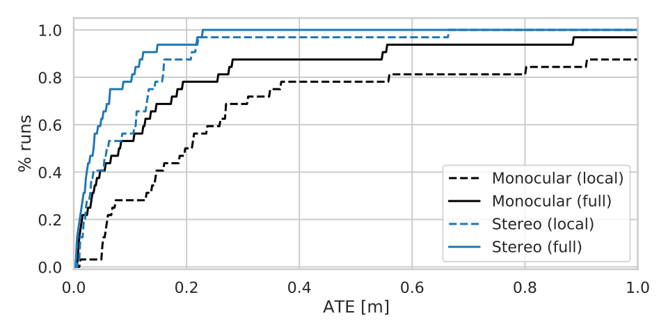
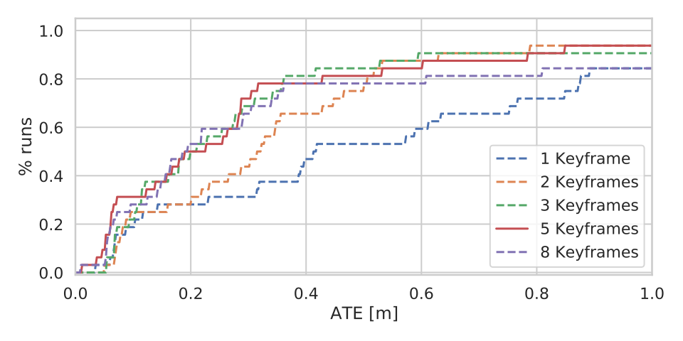
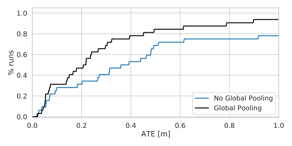
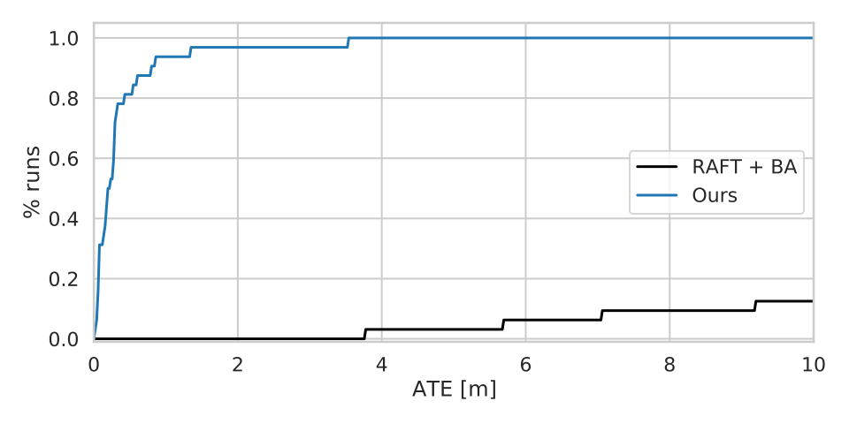
Validation ablations examine stereo observations, global optimization, local keyframe count, and pooled global context. The experiments use five local keyframes. Training the correspondence network with DBA is important: training on flow alone and adding bundle adjustment only at inference produces unstable tracking. These ablations use the TartanAir validation split.
Appendix C Camera Model and Jacobians
The appendix derives homogeneous pinhole projection, inverse-depth backprojection, and the Jacobians needed for pose and depth optimization. Local rigid-motion perturbations and the adjoint transform relate derivatives in the two camera frames; the chain rule produces the full reprojection Jacobians. The original fourteen numbered equations, including these derivations, are retained in their respective sections.
Equations 6–14
| (6) |
| (7) |
| (8) |
| (9) |
| (10) |
| (11) |
| (12) |
| (13) |
| (14) |
Appendix D Network Architecture
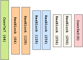
Both encoders use six residual blocks and output features at one-eighth resolution. The feature encoder uses instance normalization and 128 channels; the context encoder has no normalization and 256 channels. The update diagram shows how context, correlation, and flow features produce correspondence revisions and confidence weights.