TOQ-Nets classify events using learned relational and temporal features with explicit pooling over objects and time. Shared operations let the same network accept different object counts and sequence lengths. Experiments test few-example action learning, transfer to different player counts, and changes in event timing. The model’s logical bias improves several generalization settings, but it represents a bounded subset of temporal logic and relies on structured input features.
1 Introduction
Events such as a high soccer pass depend on relations among agents and on their ordering over time. A relational-temporal description can remain valid as the number of players or detailed timing changes. TOQ-Nets encode that idea in differentiable tensor operations: learned feature combinations express predicates, while pooling approximates finite-domain quantifiers. High-level action labels train the classifier; experiments use simulated soccer, human-activity datasets, and robot manipulation trajectories.
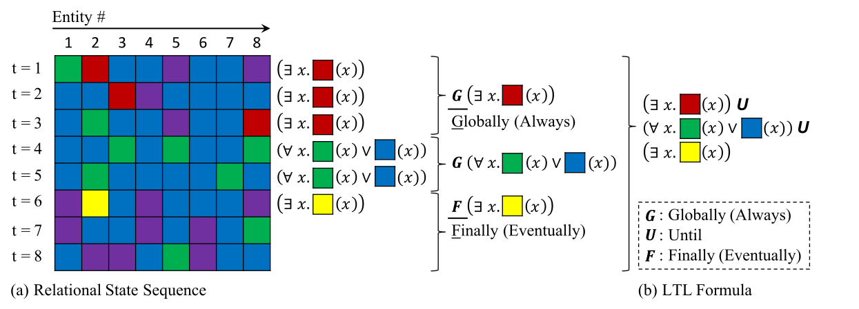
Figure 1: (a) An input sequence composed of relational states: each column represents the state of an entity that changes over time. A logic formula describes a complex concept or feature that is true of this temporal sequence using object and temporal quantification. The sequence is segmented into three stages: throughout the first stage, red holds for at least one entity, until the second stage, in which each entity is always either green or blue, until the third stage, in which yellow eventually becomes true for at least one of the entities. (b) Such events can be described using first-order linear temporal logic expressions.
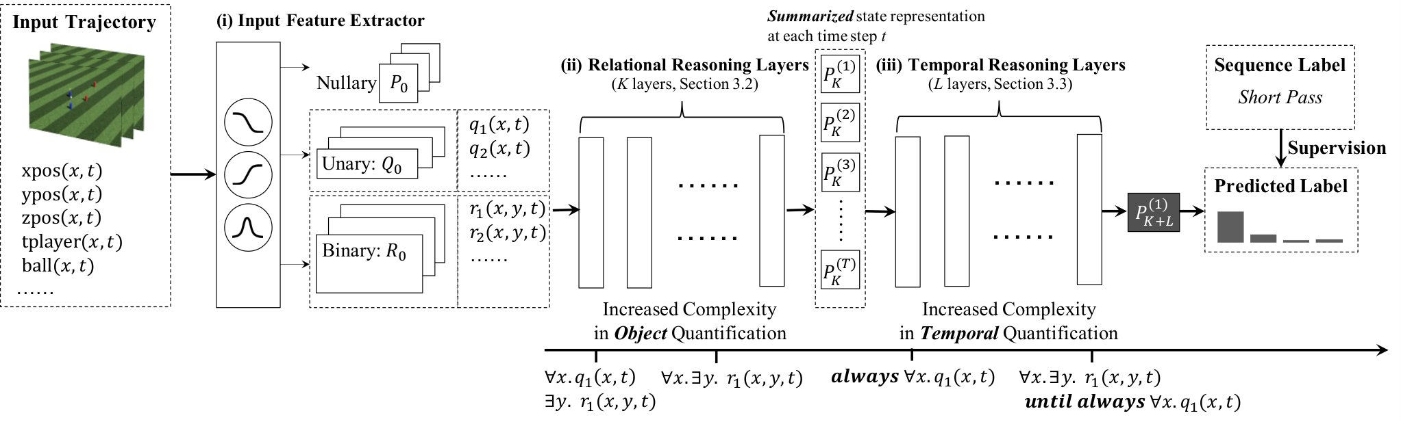
A task-specific feature extractor produces global, object, and pairwise features at each time. Relational layers combine them and pool across objects; temporal layers then summarize how the resulting events evolve. A final classifier uses the initial-time summary of the complete sequence. Quantification is over the finite objects and frames supplied to the network, and network depth bounds expression complexity. This architecture is a structural bias rather than a complete first-order temporal-logic engine.
Figure 2: A TOQ-Net contains three modules: (i) an input feature extractor, (ii) relational reasoning layers, and (iii) temporal reasoning layers.
To illustrate the model’s representational power, we show that logical forms of increasing complexity can be realized by stacking multiple layers.
2.1 Temporal-Relational Feature Representation
Nullary features describe the whole scene; unary features describe individual entities; binary features describe ordered entity pairs. Their per-frame shapes are D₀, N×D₁, and N×N×D₂. Shared transformations and reductions preserve compatibility with changing N and sequence length. Soccer inputs include entity positions and ball, target-player, and team indicators.
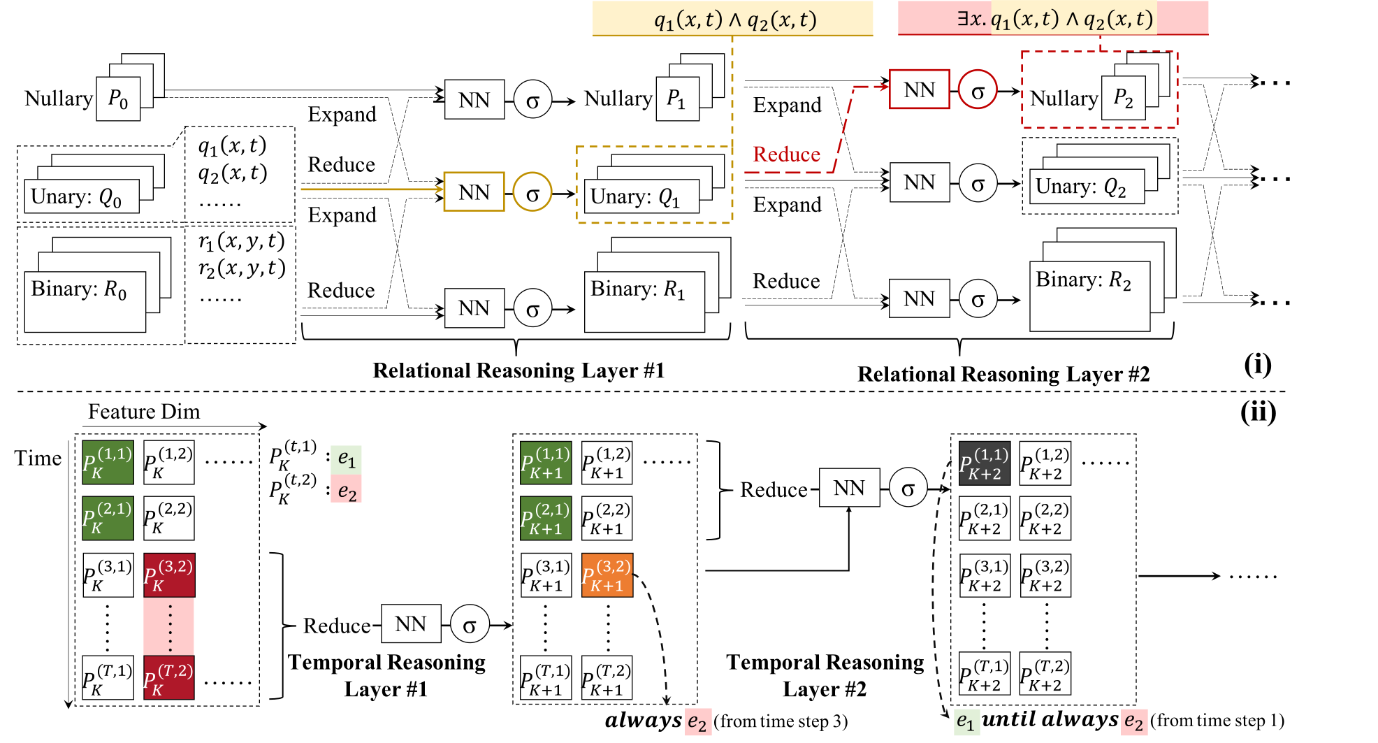
Figure 3: Illustration of (i) relational reasoning layers and (ii) temporal reasoning layers. We provide two illustrative running traces. (i) The first relational reasoning layer takes unary predicates and as input and its output is able to represent . The in layer 2 can represent .
(ii) Assume encodes the occurance of events and at each time step. The first temporal reasoning layer can realize always with a temporal pooling from time step to time step . In the second temporal reasoning layer, the temporal pooling summarizes that holds true from time step 1 to 2. Thus, the NN should be able to realize until (always ).
2.2 Relational Reasoning Layers
Following Dong et al. (2019)’s Neural Logic Machines, each relational layer combines existing features with expanded lower-arity features and max-reduced higher-arity features. Fully connected sigmoid transformations learn the feature combinations. Max reduction behaves like soft existential quantification; learned negation can express universal conditions through the same operations. Parameters are shared across entities, pairs, and frames. The experiments restrict relations to arity at most two.
Equation
2.3 Temporal Reasoning Layers
Temporal layers pool over future intervals and candidate transition times. Learned transformations combine interval summaries with events at an endpoint, enabling bounded compositions resembling always, eventually, and until. Residual connections retain earlier events. The first temporal layer is a simpler suffix-pooling operation; the worked table and algorithm show how a later layer can express p until always q. In the tested ordering, object quantification occurs inside temporal quantification, so it cannot directly express every formula that tracks the same existentially chosen object across all times. Interleaving layer types is proposed as an extension. The selected temporal construction uses quadratic space in sequence length.
Equations 1
(1)
Input
1-st Layer
2-nd Layer
G
F
G
F
U (G)
1
T
T
F
T
F
T
T
2
T
F
F
T
F
T
T
3
F
T
F
F
T
T
F
4
F
T
F
F
T
T
F
Table 1: A running example of different temporal quantification formulas that TOQ-Nets can realize. For clarity, we use T and F for True/False. In the actual computation, they are “soft” Boolean values ranges in . G means always; F means Eventually; U means until.
Algorithm 1 An example temporal structure that the second temporal reasoning layer can recognize.
1:
, , , , , and
2:
, which is true if holds true from time step until becomes always true.
3:for to do
4:for to do
5:if and then
6:
7:endif
8:endfor
9:endfor
Equations
3 Experiments
The experiments emphasize macro accuracy, scarce examples for held-out action categories, and generalization under changed object counts and timing. Standard in-distribution accuracy and robustness are reported separately.
3.1 Baseline Approaches
Baselines include STGCN (Yan et al., 2018), a max-pooling variant, a graph-plus-LSTM variant, Space-Time Region Graphs, and Non-Local Networks. Their relational and temporal operations differ. Appendix comparisons vary both capacity and input features, helping separate the proposed inductive bias from those confounds.
Table 2: Results on the soccer event dataset. Different columns correspond to different action sets (the regular, few-shot, and full action sets). The performance is measured by per-action (macro) accuracy, averaged over nine few-shot splits. The values indicate standard errors. TOQ-Net significantly outperforms all baseline methods on the few-shot action set.
Dataset and setup.
The soccer dataset uses simulator-generated trajectories and nine action categories after excluding absent or uninformative actions. Most categories have 5,000 examples, while sliding has 4,000. Each split exposes all training examples for seven regular actions and only 50 clips for each of two few-shot actions. The setup contains an internal length inconsistency: it first mentions 25-frame context, then describes ordinary 17-frame clips at 8 fps with the target action at frame 9. The later timing-shift test explicitly uses 25-frame clips.
Table 3: Results on generalization to scenarios with more agents and temporally warped trajectories on the soccer event dataset.
All models are trained only on 6v6 games. The standard errors indicated by the signs are computed with three random seeds.
Input features.
Raw entity inputs contain three-dimensional positions and four ball/player/team indicators. A Gaussian temporal indicator marks the frame of interest. The soccer feature extractor additionally computes velocities, acceleration, and pairwise distance, then learns threshold-like features; the model therefore learns predicates over supplied physical feature templates.
Results.
Across the reported nine few-shot splits, TOQ-Net achieves the strongest macro accuracy on the regular, few-shot, and combined action sets. The few-shot result supports reuse of learned relational-temporal features for categories with limited labeled clips; it is supervised low-data classification, not recognition of wholly untrained labels.
Generalization to more players.
After training on six-player teams, evaluation changes the teams to three, four, eight, or eleven players. TOQ-Net degrades less than the compared models, but still confuses unsuccessful shots with short passes when an opponent gains the ball. Shot recall falls from 97% to 60% in the described larger-team analysis. This exposes a limitation of outcome-based physical cues without a representation of player intent.
Generalization to temporally warped trajectories.
Timing tests place the sole target action between frames 6 and 19 in a 25-frame clip. Temporal convolution and LSTM baselines lose substantial accuracy; TOQ-Net retains much more. Space-Time and Non-Local models change little under this shift partly because they are insensitive to temporal ordering, so invariance alone should not be read as evidence of detailed temporal reasoning.
3.3 Extension to Real-World Datasets
The real-world experiments use structured skeleton or annotated player inputs rather than raw-video recognition.
3.3.1 Toyota Smarthome
Toyota Smarthome provides about 16,100 videos in 19 classes. Thirty sampled frames supply joint positions, velocities, limb lengths, and angles. Standard accuracy is similar: TOQ-Net 42.0%, STGCN 43.0%. Under doubled-speed sequences, TOQ-Net retains 41.2% while STGCN falls to 32.3%, illustrating robustness without an in-distribution accuracy advantage.
3.3.2 Volleyball Activity
The volleyball experiment uses 4,830 clips, eight group-activity classes, and manual player boxes, involvement indicators, and individual-action annotations as inputs. Standard accuracy is 73.3% for TOQ-Net and 73.6% for STGCN. Under temporal shifts and doubled speed, TOQ-Net scores 70.3% and 70.7%, versus 39.5% and 48.6%. These results depend on the substantial structured annotations supplied to the classifiers.
4 Related Work
Action concept representations and learning.
Symbolic activity models can express temporal relations but often require annotated primitives, rules, or combinatorial search. TOQ-Nets replace explicit rule search with gradient-trained feature combinations and quantification operations.
Temporal and relational reasoning.
Related approaches include temporal-logic learners, logical neural networks, hidden-state models, graph networks, and recurrent models. TOQ-Nets share structured relational inputs with several baselines but use a different temporal aggregation mechanism.
5 Conclusion and Discussion
Pooling-based object and time quantification can improve generalization across entity counts and temporal variation. Remaining limits include restricted logical expressiveness, dependence on task-specific physical or annotated features, quadratic temporal computation, and ambiguity about goals or intentions. Broader transfer between object kinds and integration of mental-state variables remain future work.
Acknowledgements
The authors thank Tomás Lozano-Pérez and acknowledge the listed research sponsors.
Supplementary Material for Temporal and Object Quantification Networks
The supplement adds robot-manipulation evaluation, complete model and training specifications, capacity and input-feature comparisons, scale-transfer experiments, and interpretability examples.
Appendix A Manipulation Concept Learning from 6D Poses
The manipulation setting tests whether temporal-relational representations transfer beyond soccer into object interactions by a robot arm.
Dataset and setup.
RLBench generates 100 trajectories for each of 24 manipulation actions, with randomized object poses and built-in motion planning. Lengths range from 30 to 1,000 frames, usually near 50. The stated split is 60% training, 15% validation, and 25% test. The subsequent input paragraph says regular actions average 65 training trajectories; this differs from the stated 60-example training split.
Input.
Objects are represented by position, quaternion orientation, and axis-aligned box coordinates; the robot gripper includes pose and an open/closed indicator. Articulated or deformable items are split into meaningful pieces, such as a separate box lid. These structured state inputs carry information unavailable from raw images alone.
Input features.
TOQ-Net adds a learned sigmoid projection of the raw state vectors. The recurrent baseline uses temporal kernel size one in its graph front end, isolating the LSTM’s contribution; the supplement also compares kernel size three.
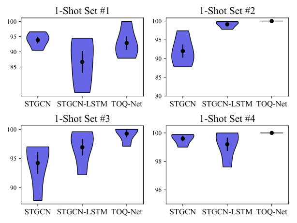
Table 1: Few-shot learning on the RLBench dataset, measured by per-action (macro) accuracy and averaged of four 1-shot splits and four random seeds per split. The values indicate standard errors. On the right we shows the sampled performance of different models on each individual 1-shot split.
l
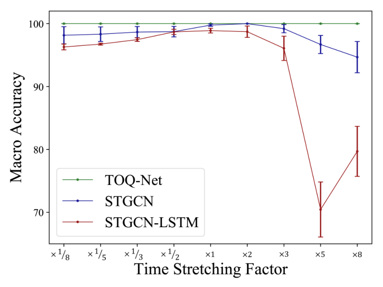
Figure 1: Comparing different models with different time stretching factors on the RLBench dataset.
Results.
The 24-way experiment stretches trajectories from one-eighth to eight times their original duration. The retained plot shows TOQ-Net’s strong performance across these changes compared with convolutional and recurrent baselines.
Generalization to new action concepts.
A one-shot protocol withholds half the opening and closing action types, providing one example of each held-out type. Classification groups them as Open-X, Close-X, or Other. Performance varies across splits: closing jars and drawers is harder, plausibly because rotation or pushing differs from other closing motions. The test concerns learning with one example of a new type, not zero-shot object transfer.
The implementation section specifies three object and three temporal layers, with relational/temporal widths 16/48 for soccer and 48/144 for manipulation. A later depth study recommends three relational and four temporal layers; the source does not reconcile those two specifications.
Input feature extractor.
Soccer features derive ground speed, vertical speed, acceleration, and pairwise distance from trajectories. Each normalized physical property produces five trainable sigmoid-threshold features; the temperature decays from 1 to 0.001. Manipulation instead uses a 64-dimensional sigmoid linear projection. The thresholds are learned, while the physical feature family is designed.
STGCN follows the cited architecture, with the complete layer specification retained. Average pooling over time and entities yields a 256-dimensional classification feature.
Input feature extractor.
The original soccer STGCN cannot consume pairwise-distance predicates, unlike TOQ-Net. Manipulation input formats are shared. The separate STGCN-2D experiment checks whether supplying binary features closes the gap.
STGCN-MAX changes neighbor aggregation from averaging to elementwise maxima, making its relational update closer to the proposed model while retaining temporal convolutions.
STGCN-2D adds binary inputs such as distance. It improves standard and few-shot soccer accuracy somewhat but does not recover TOQ-Net’s generalization to different player counts or shifted timing. Both complete comparison tables are retained.
Table 3: Ablation study of the STGCN-2D model on the soccer event dataset, evaluated by its generalization to different number of players and time-warped trajectories.
STGCN-LSTM pools graph features over entities and passes the resulting sequence to a two-layer bidirectional LSTM with hidden width 256. Soccer uses temporal kernel size three and manipulation size one, both at stride one. The manipulation ablation finds similar performance for kernel sizes one and three.
B.6 Space-Time Region Graph Networks
Space-Time Region Graphs use the cited graph-convolutional formulation. The full architectural table preserves each layer and its dimensions.
B.7 Non-Local Neural Networks
Non-Local Networks apply attention over the same space-time graph instead of graph convolution. The full layer specification is retained.
Table 4: Ablation study of different kernel sizes for the STGCN-LSTM model on the RLBench dataset, measured by per-action (macro) accuracy and averaged of four 1-shot splits and four random seeds per split. The values indicate standard errors.
Soccer event detection.
Soccer batches contain 128 examples, balanced by first sampling an action category. Adam starts at 0.002, remains fixed for 50 epochs, then decays by 0.9 after six epochs without improved validation loss; training lasts 200 epochs. The separate input-scale adaptation task fine-tunes pretrained models for 10,000 iterations using a small new dataset.
Manipulation concept learning.
Manipulation training uses Adam at 0.003 with the analogous plateau schedule for 150 epochs. Batch sizes differ: 32 for STGCN-based models and four for TOQ-Net.
Table 5: The STGCN architecture used in the paper.
Model
Input Dim.
Output Dim.
Stride
Residual
Space-Time
-
64
1
False
64
64
1
True
64
64
1
True
64
64
1
True
64
128
2
True
128
128
1
True
128
128
1
True
128
256
2
True
256
256
1
True
256
256
1
True
Space-TimeS
-
16
1
False
16
16
1
True
16
32
2
True
32
64
2
True
64
128
1
True
Space-TimeT
-
32
1
False
32
64
2
True
64
64
2
True
Table 6: The Space-Time Region Graph architecture used in the paper.
Model
Input Dim.
Output Dim.
Stride
Residual
Non-Local
-
64
1
False
64
64
1
True
64
64
1
True
64
64
1
True
64
128
2
True
128
128
1
True
128
128
1
True
128
256
2
True
256
256
1
True
256
256
1
True
Non-LocalS
-
32
1
False
32
32
2
True
32
64
2
True
64
128
1
True
Non-LocalT
-
32
1
False
32
32
2
True
32
64
2
True
Table 7: The Non-local Neural Networks architecture used in the paper.
Appendix C Additional Ablation Study
C.1 Network Architecture
Capacity ablations compare original, small, and tiny baselines. Most best-performing variants are smaller; main comparisons use the selected best variant for each baseline. TOQ-Net has about 35,000 parameters and still leads the reported soccer few-shot comparison.
Table 8: Results on the soccer event dataset for baselines with different capacities, where modelS and modelT denote the small and the tiny variant for each model. The performance is measured by per-action (macro) accuracy, averaged over nine few-shot splits. The values indicate standard errors. For each baseline we showed the best performance over three levels of capacities. In fact, performances of most of the models are not affected much by the capacity. We highlight the best-performing variants of all baselines, and use them in all comparisons in the main text.
C.2 Generalization to different input scales
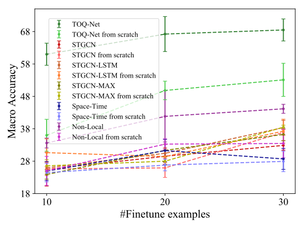
A separate adaptation experiment enlarges the soccer field and changes temporal/spatial scale. All models are pretrained on the original nine-class task, then fine-tuned with few examples from the changed setting. TOQ-Net benefits especially when that adaptation set is small. These curves measure sample-efficient adaptation, unlike the direct player-count transfer test.
Figure 2: Generalization to soccer environments with a different court size and agent speeds. The standard errors are computed based on three random seeds.
C.3 Full Results for the Time-Warping Generalization
The full table crosses all five tested team sizes with the timing-shift condition, retaining each model’s accuracy and relative degradation.
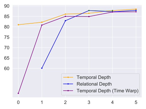
The depth study shows that relational layers are required to aggregate entity-only inputs and that temporal layers support timing robustness. The plot recommends three relational and four temporal layers as a computation/performance tradeoff, while the earlier implementation paragraph states three of each.
C.5 Interpretability
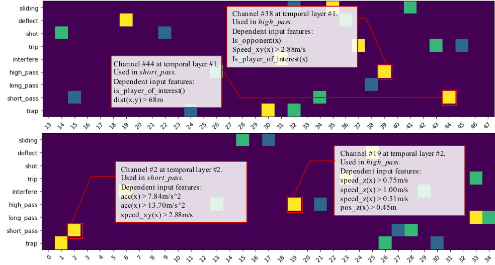
Gradient-based dependency plots trace learned feature channels supporting high-pass and short-pass predictions. They illustrate compositional use of low-level properties, but are qualitative explanations rather than proof that every feature has a stable symbolic interpretation.
Table 9: Full results on generalization to scenarios with all combinations of #agents and temporally warping on the soccer event dataset. The standard error of all values are smaller than 2.5%, computed based on three random seeds.
Figure 3: Comparing # of reasoning layers. Accuracy is tested on 6v6 9-way classification. When # of relational reasoning layers vary (blue), temporal reasoning layers are fixed at 4. When # of temporal reasoning layers vary (orange), relational reasoning layers are fixed at 3. When we have 0 temporal reasoning layers, we predict the sequence label based on the feature of the frame of interest. The purple line shows the performance on temporally warped trajectories when we have the # of relational reasoning layers fixed and vary the # of temporal reasoning layers. Relational layers are required for the prediction task (# of relational reasoning layer must be greater than 0), because there is no nullary feature input to the network: we need at least one relational reasoning layer to gather information across the entities. Overall, adding reasoning layers improves results, and 3 relational layers + 4 temporal layers is a good balance between computation and performance. Figure 4: Relevant features in temporal layers. Feature dependencies are computed by gradient. These dependencies and thresholds are learned end-to-end from data. Insets detail features for events in the first and the second stage of the high pass and short pass.
34 references
Baker et al. [2017]
Chris L Baker, Julian Jara-Ettinger, Rebecca Saxe, and Joshua B Tenenbaum.
Rational quantitative attribution of beliefs, desires and percepts in
human mentalizing.
Nature Human Behaviour, 1(4):1–10, 2017.
Battaglia et al. [2018]
Peter W Battaglia, Jessica B Hamrick, Victor Bapst, Alvaro Sanchez-Gonzalez,
Vinicius Zambaldi, Mateusz Malinowski, Andrea Tacchetti, David Raposo, Adam
Santoro, Ryan Faulkner, et al.
Relational inductive biases, deep learning, and graph networks.
arXiv:1806.01261, 2018.
Bruna et al. [2014]
Joan Bruna, Wojciech Zaremba, Arthur Szlam, and Yann LeCun.
Spectral networks and locally connected networks on graphs.
In ICLR, 2014.
Chou et al. [2020]
Glen Chou, Necmiye Ozay, and Dmitry Berenson.
Explaining multi-stage tasks by learning temporal logic formulas from
suboptimal demonstrations.
In RSS, 2020.
Das et al. [2019]
Srijan Das, Rui Dai, Michal Koperski, Luca Minciullo, Lorenzo Garattoni,
Francois Bremond, and Gianpiero Francesca.
Toyota smarthome: Real-world activities of daily living.
In ICCV, 2019.
Deng et al. [2016]
Zhiwei Deng, Arash Vahdat, Hexiang Hu, and Greg Mori.
Structure inference machines: Recurrent neural networks for analyzing
relations in group activity recognition.
In CVPR, 2016.
Ibrahim et al. [2016]
Mostafa S. Ibrahim, Srikanth Muralidharan, Zhiwei Deng, Arash Vahdat, and Greg
Mori.
A hierarchical deep temporal model for group activity recognition.
In CVPR, 2016.
Lamb et al. [2007]
Luis C. Lamb, Rafael V. Borges, and A. d’Avila Garcez.
A connectionist cognitive model for temporal synchronisation and
learning.
In AAAI, 2007.
Penning et al. [2011]
Leo de Penning, A. d’Avila Garcez, Luís C. Lamb, and John-Jules C. Meyer.
A neural-symbolic cognitive agent for online learning and reasoning.
In IJCAI, 2011.
Qi et al. [2018]
Mengshi Qi, Jie Qin, Annan Li, Yunhong Wang, Jiebo Luo, and Luc Van Gool.
stagnet: An attentive semantic rnn for group activity recognition.
In ECCV, 2018.
Stränger and
Hommel [1996]
Jürgen Stränger and Bernhard Hommel.
The perception of action and movement.
In Handbook of perception and action, volume 1, pages 397–451.
Elsevier, 1996.
Vallacher and
Wegner [1987]
Robin R Vallacher and Daniel M Wegner.
What do people think they’re doing? action identification and human
behavior.
Psychol. Rev., 94(1):3, 1987.
Yan et al. [2018]
Sijie Yan, Yuanjun Xiong, and Dahua Lin.
Spatial temporal graph convolutional networks for skeleton-based
action recognition.
In AAAI, 2018.
Zacks et al. [2001]
Jeffrey M Zacks, Barbara Tversky, and Gowri Iyer.
Perceiving, remembering, and communicating structure in events.
J. Exp. Psychol. Gen., 130(1):29, 2001.
Zacks et al. [2007]
Jeffrey M Zacks, Nicole K Speer, Khena M Swallow, Todd S Braver, and Jeremy R
Reynolds.
Event perception: a mind-brain perspective.
Psychol. Bull., 133(2):273, 2007.
James et al. [2020]
Stephen James, Zicong Ma, David Rovick Arrojo, and Andrew J. Davison.
Rlbench: The robot learning benchmark & learning environment.
RA-L, 2020.
Yan et al. [2018]
Sijie Yan, Yuanjun Xiong, and Dahua Lin.
Spatial temporal graph convolutional networks for skeleton-based
action recognition.
In AAAI, 2018.