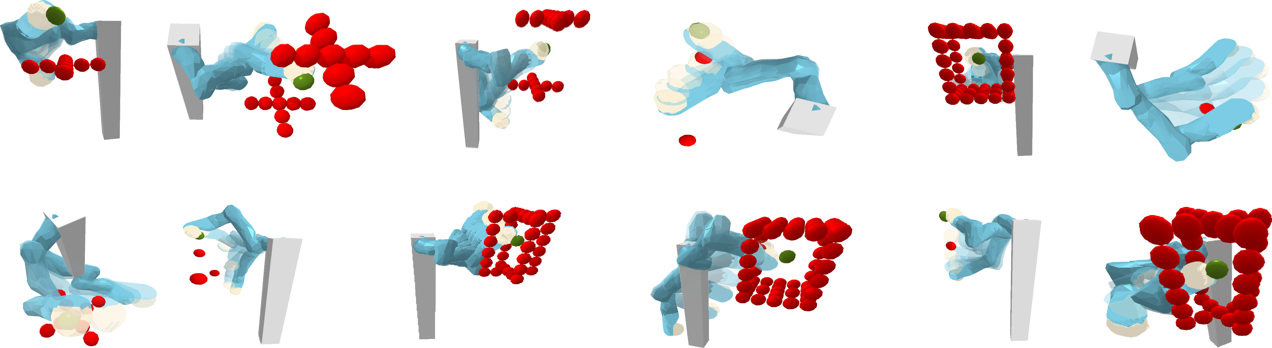
Fig. 1: Composable Energy Policies generate trajectories reactively in a wide set of environments, as the ones in the figure. The generated trajectories are attracted to a target pose, visualized by the green sphere, and avoid a set of obstacles, shown as red spheres.
At a glance
Composable Energy Policies (CEP) select robot actions by maximizing a product of stochastic component policies. This can retain several acceptable actions for each objective, instead of combining independently chosen deterministic actions that may conflict. An energy tree brings objectives from different task spaces into a common optimization, and a hierarchical variant combines fixed priors with reinforcement learning. Experiments improve reactive reaching and puck-hitting performance, while difficult cages and long-horizon conflicts remain limitations.
I Introduction
Reaching a target, avoiding obstacles, and respecting joint limits must often be satisfied simultaneously. Global planning reasons over trajectories but costs more computation; reactive controllers respond quickly but can oscillate or become trapped. CEP seeks actions jointly favored by all components. Multiplying policy distributions acts like a probabilistic conjunction, allowing multiple acceptable avoidance directions to survive until the objectives are combined. [20][32]
Equation 1
(1)
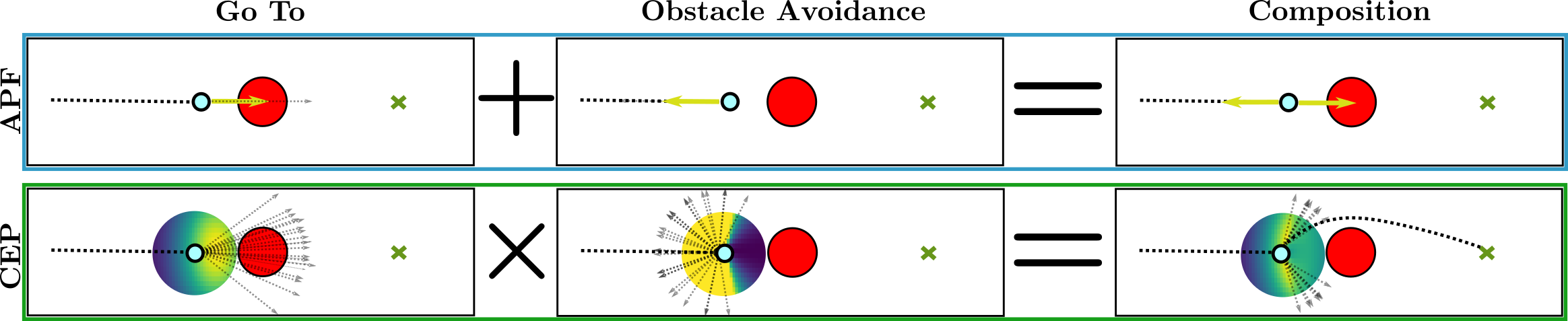
Fig. 2: Visual Representation of modular control for Goto + Obstacle Avoidance. In the top box, we show Artificial Potential Field (APF) [20] policy. In the bottom box, we show Composable Energy Policies (CEP). In contrast, with artificial potential field method, that sums deterministic actions (goto, avoid obstacle), CEP computes the product of the policy distributions. The composition will provide high probability to those actions that satisfy both components and low to the rest. This approach helps avoiding conflicts between different components. Robot: blue circle, obstacle: red circle and target: green cross. Thick dotted line: performed trajectory, light dotted line: possible future trajectories.
Contribution
The contribution is a modular energy representation, optimization over its composed policy, and a hierarchical learning interface for priors from different sources. The appendix relates composition to control as inference and explains why locally combined objectives need not recover a globally optimal trajectory. Hard-constraint behavior requires suitable priors and successful optimization; the empirical method is not a general collision-free planning guarantee.
Notation
Superscripts identify the space in which a policy is represented, subscripts identify policy components, and mapping functions transform states and actions between configuration and task spaces.
II Preliminaries
II-A Artificial Potential Fields
Artificial potential fields combine task-space dynamical systems into a robot action through weighted projections. Independently preferred accelerations can conflict. CEP replaces each deterministic proposal with an energy distribution over possible actions, then selects an action from the combined objective. Gaussian component energies recover a form of potential-field composition, while richer energies can represent constraints and multiple suitable directions.
Equation 2
(2)
III Composable Energy Policies
A Boltzmann policy assigns probability proportional to an exponentiated energy. A weighted product of policies becomes a weighted sum of energies in log space. Normalizing constants independent of the candidate action need not be computed for action selection, and components can be evaluated in parallel.
Equations 3–4
(3)
(4)
III-A Energy Tree
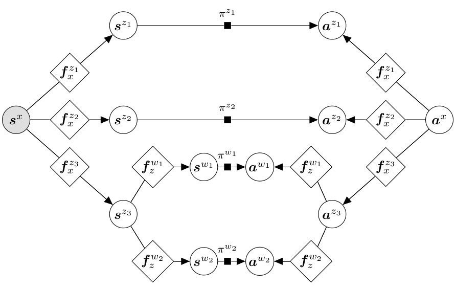
An energy tree maps a candidate configuration-space action into each component’s task space, evaluates the corresponding energies, and combines them. The resulting controller is implicit: it optimizes a score instead of directly mapping each component’s preferred action back through an inverse. The paper’s density change-of-variables equality requires bijective action maps; its extension to injective or surjective maps is a practical approximation explicitly left for further study.
Equations 5–10
(5)
(6)
(7)
(8)
(9)
(10)
Fig. 3: Bayesian network for the energy tree. The policy distribution is computed w.r.t. the policies in the latent spaces . Additionally, a latent policy can be represented by a set of policies in a different latent spaces . White diamonds represent deterministic transformations and black square is a probabilistic mapping.
Cross-entropy optimization repeatedly samples candidate actions, scores their combined energies, and updates a proposal distribution. Algorithm 1 preserves the complete procedure. Batched GPU evaluation of candidates and independent components makes this stochastic search practical at the reported control frequencies.
Equations 11–12
(11)
(12)
Algorithm 1Composable Energy Policies
Given : : Number of samples;
: Current state in common space;
: Number of Energy Components;
: Maps, energies and inverse temperatures;
: Optimization steps;
: Initial sampling distribution mean and variance;
Robot state is joint position and velocity, and the action is joint acceleration. Forward kinematics and Jacobians map candidates to task-space accelerations. The approach avoids explicitly inverting the task map during action selection, although its performance still depends on the chosen energies and numerical search.
Equations 13–15
(13)
(14)
(15)
Go To a target
A Gaussian goal-reaching policy is centered on a proportional–derivative controller. Its covariance shrinks with distance to the target, making the goal component increasingly selective near the desired state.
Equations 16–18
(16)
(17)
(18)
Obstacle Avoidance
Obstacle avoidance projects velocity and acceleration onto the robot-to-obstacle direction. Far from an obstacle, or while moving away, the component is unrestrictive. Close to an obstacle while approaching it, the allowed acceleration interval enforces braking away from the obstacle. This represents a set of acceptable actions rather than a single repulsive vector.
Equations 19–21
(19)
(20)
(21)
Avoid Joint Limits
A similar interval-based energy activates near joint limits and favors accelerations directed back toward the allowed region. The displayed equations retain the distance, activation threshold, and braking parameters.
Component distributions can also come from imitation learning, probabilistic control inference, or reinforcement learning. Multimodal policies are allowed; the architecture is not limited to Gaussian heuristic controllers.
The high-level learned policy supplies the mean and covariance of a Gaussian component, which the low-level CEP optimizer combines with fixed priors. A prior can exclude actions by assigning zero probability or encourage exploration in several regions. The learned covariance controls how strongly the new policy competes with these priors.
This differs from adding an unrestricted residual to a safe action: composition can preserve explicit exclusions represented by the prior. In practice, numerical optimization, prior validity, and the covariance choice matter; the ablation observes more collisions when the learned component reduces the prior’s influence.
Equations 24–26
(24)
(25)
(26)
VI Experimental Evaluation
Evaluation separates reactive motion generation from prior-guided learning. Comparisons target reactive controllers rather than global planners, and the learning comparison uses the same prior across methods.
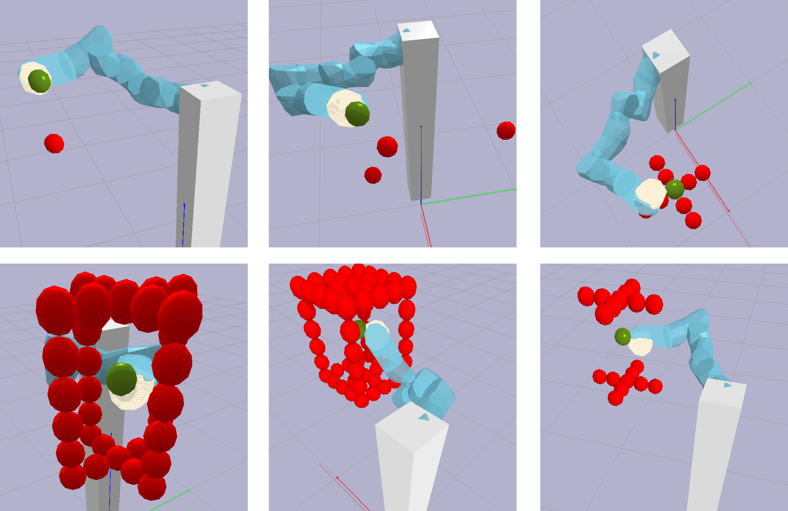
Fig. 4: Reactive Motion Generation Environments. In the top, from left to right: 1 Obstacle, 3 Obstacles, Cross. In the bottom, from left to right: Cage I, Cage II, Double Cross. Green Sphere: target pose, red spheres: obstacles.
Reactive Motion Generation
A seven-degree-of-freedom KUKA-LWR arm reaches position-only or full-pose targets in increasingly difficult obstacle arrangements. CEP combines target, link-obstacle, and joint-limit energies and is compared with potential fields and Riemannian motion policies. The reported implementation evaluates 10,000 action candidates per search step and uses two steps with GPU parallelization to target control at at least 500 Hz.
TABLE II: Results for 6D GoTo + Obstacle Avoidance Task
Results and analysis
For position reaching, CEP succeeds in 89 of 100 trials in Cage I and 46 in Cage II, compared with 55/5 for RMP and 43/4 for potential fields. No CEP collisions are recorded in these trials. Full-pose reaching is harder: CEP’s cage success falls to 43% and 14%. It still exceeds the tested baselines but frequently fails to reach the goal, supporting the need for a global planner in difficult environments.
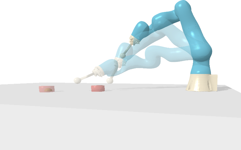
Fig. 5: Puck hitting environment. CEP is tested in a RL environment where the robot needs to learn how to hit the puck. The reward is defined by the euclidean distance between the puck and the green target. An additional reward penalizes if the robot hits the table.
A seven-degree-of-freedom arm must strike a puck toward a target while avoiding the table. The learned action is three-dimensional end-effector velocity. PPO compares behavior-cloning initialization, additive residual learning, and CEP composition, all using the same goal-reaching/table-avoidance prior. Rewards combine puck-target distance with a large table-collision penalty. [37][39]
Equations 27–33
(27)
(28)
(29)
(30)
(31)
(32)
(33)
Results and analysis
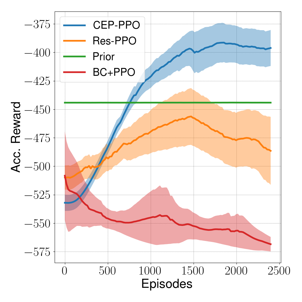
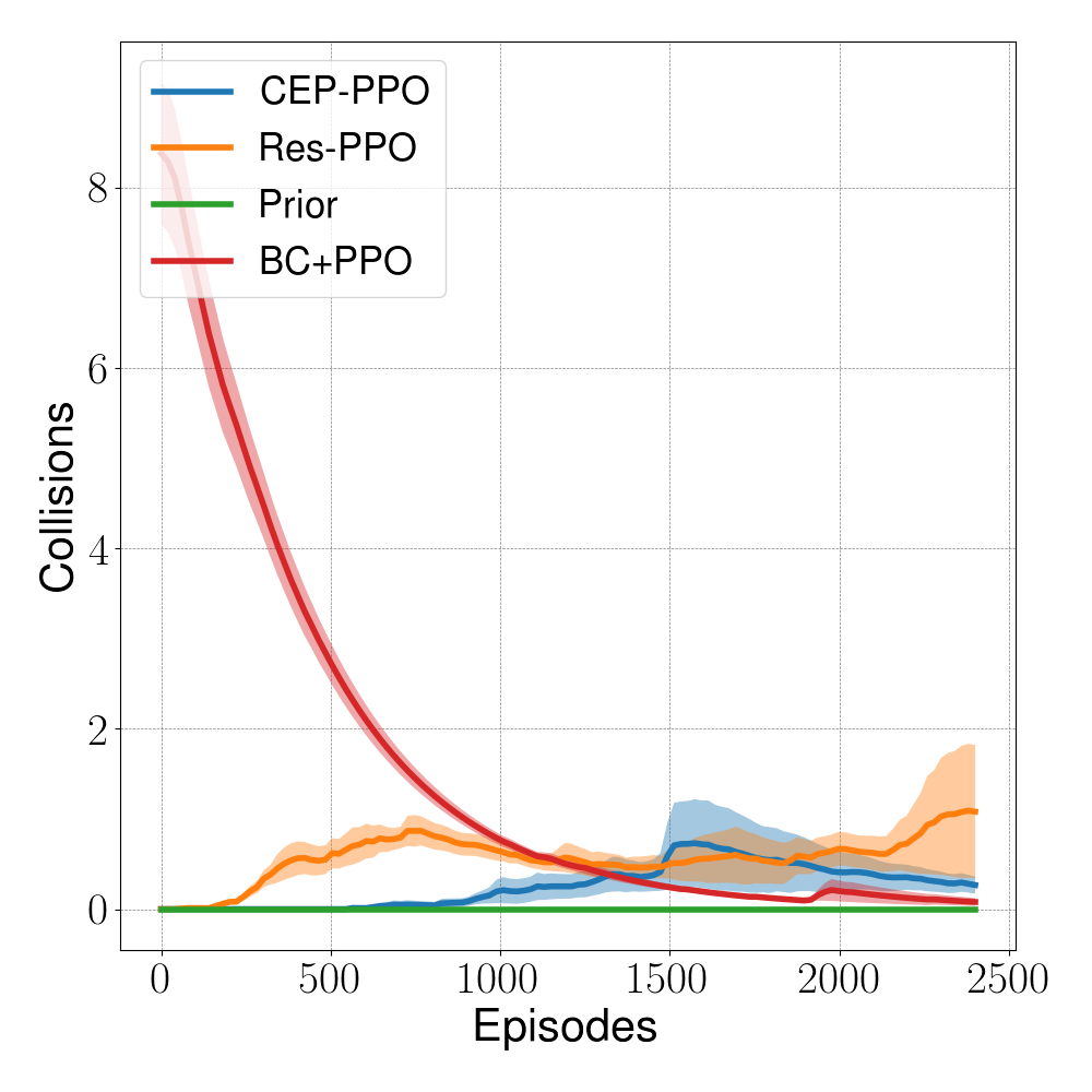
CEP-PPO improves reward more consistently and records fewer table collisions than the tested alternatives. The behavior-cloned policy can learn to avoid the table by abandoning useful striking behavior, while unrestricted residual actions disturb the prior’s avoidance behavior. The result supports preserving useful prior constraints during exploration rather than treating the comparison as a universal ranking of learning algorithms.
Fig. 6: Training curves for Hitting a puck environment. CEP-PPO performs consistenly better than other prior + RL methods. Collision avoidance prior is stronger in CEP-PPO and provides a safer training.
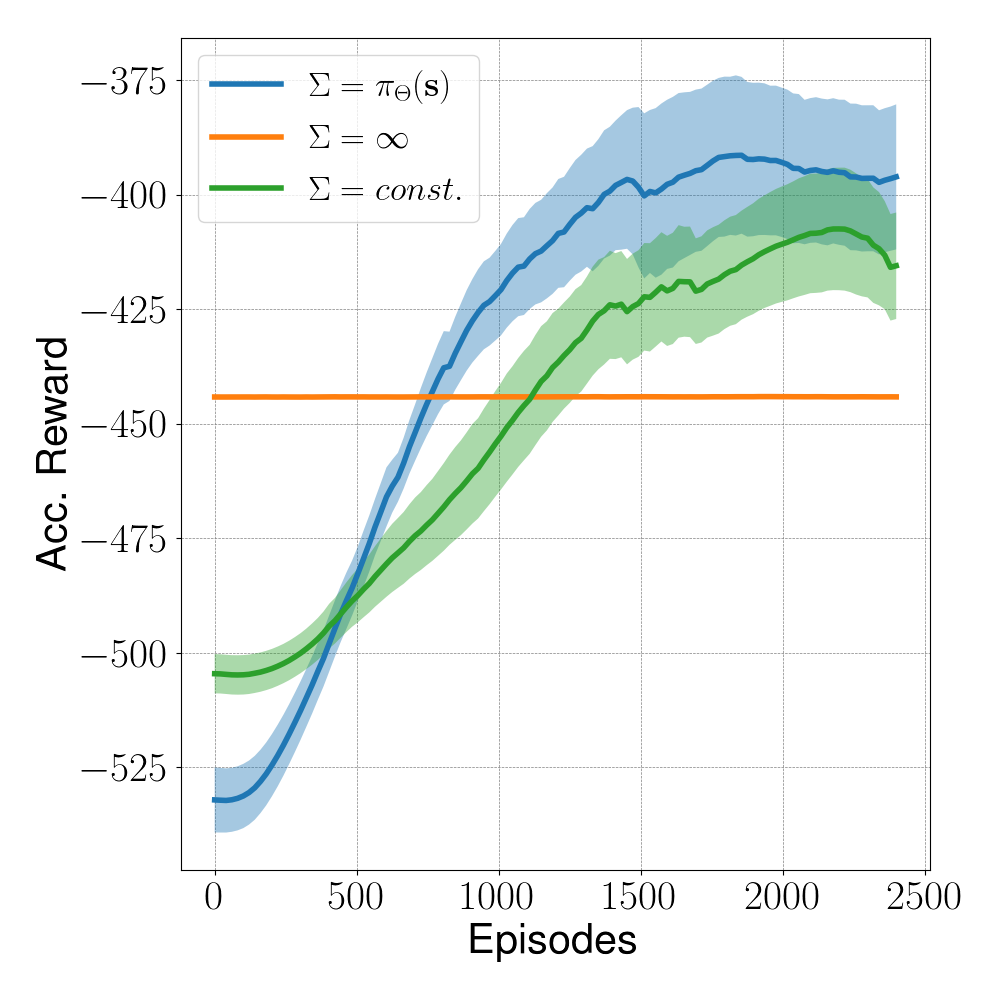
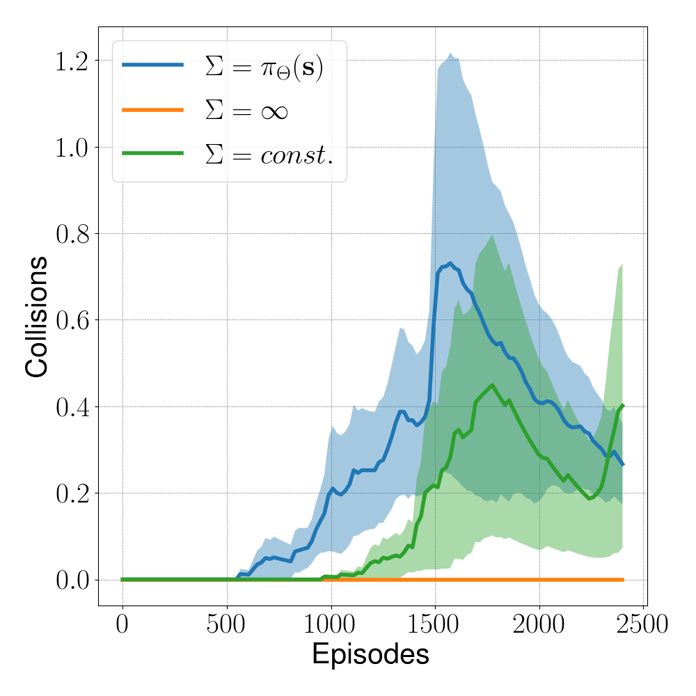
Learning the Gaussian covariance outperforms the tested fixed-covariance choices in reward. A large fixed covariance lets the prior dominate; a small one gives the learned policy more influence. Adapting this tradeoff improves hitting behavior but can increase collisions, so the most flexible variant does not provide unconditional safety.
Fig. 7: Training curves for Hitting a puck environment. Learning the variance of the policy improves the learning curve, but also increases the probability of collisions.
VII Conclusions
CEP provides a common optimization interface for simultaneously active motion objectives and learned priors. Its benefits come from retaining distributions over acceptable actions before composition. The experiments support improved local control, while incomplete cage success, long-horizon interactions, and approximate treatment of non-bijective mappings limit stronger claims.
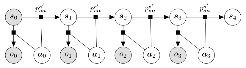
Appendix A A Control as Inference view for Reactive motion generation
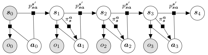
Control as inference introduces optimality variables whose likelihood depends on reward, producing a posterior over action trajectories. A reactive controller instead optimizes only the next action, integrating over future states and actions under an assumed future policy. Its local energy depends on that policy’s action-value function; global optimality requires an appropriate optimal value function, not merely a short computation horizon.
Fig. 8: Graphical model for the Optimal Control problem. denoted the state, denotes the action and is an additional variable representing the optimality of the state and action for a given reward.
Equations 34–37
(34)
(35)
(36)
(37)
Fig. 9: Graphical model for one-step ahead optimal control problem. In this approach, the actions are dependant on given a policy .
Equations 38–39
(38)
(39)
A-A Optimality Guarantees
The sum of independently optimal component action-value functions generally differs from the optimal value for the combined reward. The derivation recovers equality for the one-step case and analyzes how disagreement accumulates over longer horizons. Identical component values eliminate the composition discrepancy; conflicting objectives increase it. The retained recurrence and related maximum-entropy bounds explain why reactive composition becomes less reliable when success depends on long-term coordination.
Equations 40–54
(40)
(41)
(42)
(43)
(44)
(45)
(47)
(48)
(49)
(50)
(51)
(52)
(53)
(54)
Appendix B Composable Energy Policies as Inference
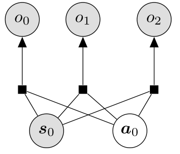
Independent optimality factors conditioned on the same state and action yield a posterior proportional to the product of their likelihoods and an action prior. With a uniform prior, maximizing this posterior recovers the summed-energy CEP objective. This is an alternative interpretation of the energy tree’s product of policies.
Fig. 10: Graphical model for Composable Energy Policies. is an auxiliary variable that represents the optimality of and for a particular energy.Equations 55–56
(55)
(56)
Appendix C Composable Energy Policies and Artificial Potential Fields Method
If all components are Gaussian, their product is Gaussian and its maximizer is a precision-weighted combination of component means. This recovers a potential-field-style acceleration rule. Gaussian assumptions are restrictive for avoidance: several qualitatively different actions may be safe, and quality need not decay smoothly with distance from a single preferred action.
Equations 57–64
(57)
(58)
(59)
(60)
(61)
(62)
(63)
(64)
Appendix D Experiments
D-A Reactive Motion Generation
Table III preserves the goal-attraction gains and covariance scale, plus obstacle and joint-limit activation/braking parameters. Baseline components follow the cited potential-field and RMPflow formulations. [3]
Energy Modules
Parameters
Reach Target
Obstacle Avoidance
Joint Limits avoidance
TABLE III: Component parameters for Composable Energy Policies in reactive motion generation
Table IV retains the shared PPO networks and optimization settings, including a 1,400-step horizon, discount factor 0.997, and separate actor/critic learning rates. The same settings are used for the three prior-based learning methods.
Hyperparameters
horizon
1400
Policy Net
18-128-128-3
policy std0
1.
policy batch
256
n_epochs_policy
2
policy learn rate
1e-4
Critic Net
18-256-256-1
critic batch
256
critic learn rate
3e-4
n_steps_per_fit
horizon x 30
Discount factor
.997
TABLE IV: Component parameters for Composable Energy Policies in reactive motion generation
50 references
[1]
Adi Ben-Israel.
The change-of-variables formula using matrix volume.
SIAM Journal on Matrix Analysis and Applications, 21(1):300–312, 1999.
[3]
Ching-An Cheng, Mustafa Mukadam, Jan Issac, Stan Birchfield, Dieter Fox, Byron
Boots, and Nathan Ratliff.
Rmpflow: A computational graph for automatic motion policy
generation.
In International Workshop on the Algorithmic Foundations of
Robotics, 2018.
[5]
Christian Daniel, Gerhard Neumann, and Jan Peters.
Hierarchical relative entropy policy search.
In Artificial Intelligence and Statistics, pages 273–281.
PMLR, 2012.
[6]
Carlo D’Eramo, Davide Tateo, Andrea Bonarini, Marcello Restelli, and Jan
Peters.
Mushroomrl: Simplifying reinforcement learning research.
https://github.com/MushroomRL/mushroom-rl, 2020.
[7]
Yilun Du, Shuang Li, and Igor Mordatch.
Compositional visual generation and inference with energy based
models.
In Conference on Neural Information Processing Systems, 2020.
[8]
Carlos Florensa, Yan Duan, and Pieter Abbeel.
Stochastic neural networks for hierarchical reinforcement learning.
In International Conference on Learning Representations, 2017.
[11]
Tuomas Haarnoja, Vitchyr Pong, Aurick Zhou, Murtaza Dalal, Pieter Abbeel, and
Sergey Levine.
Composable deep reinforcement learning for robotic manipulation.
In IEEE International Conference on Robotics and Automation,
pages 6244–6251. IEEE, 2018.
[12]
Nicolas Heess, Greg Wayne, Yuval Tassa, Timothy Lillicrap, Martin Riedmiller,
and David Silver.
Learning and transfer of modulated locomotor controllers.
arXiv preprint arXiv:1610.05182, 2016.
[14]
Andrew Howard, Maja J Matarić, and Gaurav S Sukhatme.
Mobile sensor network deployment using potential fields: A
distributed, scalable solution to the area coverage problem.
In Distributed Autonomous Robotic Systems 5, pages 299–308.
Springer, 2002.
[15]
Tobias Johannink, Shikhar Bahl, Ashvin Nair, Jianlan Luo, Avinash Kumar,
Matthias Loskyll, Juan Aparicio Ojea, Eugen Solowjow, and Sergey Levine.
Residual reinforcement learning for robot control.
In International Conference on Robotics and Automation, pages
6023–6029. IEEE, 2019.
[16]
Leslie Pack Kaelbling and Tomás Lozano-Pérez.
Hierarchical task and motion planning in the now.
In IEEE International Conference on Robotics and Automation,
pages 1470–1477. IEEE, 2011.
[17]
Leslie Pack Kaelbling and Tomás Lozano-Pérez.
Integrated task and motion planning in belief space.
The International Journal of Robotics Research, 32(9-10):1194–1227, 2013.
[18]
Mrinal Kalakrishnan, Sachin Chitta, Evangelos Theodorou, Peter Pastor, and
Stefan Schaal.
Stomp: Stochastic trajectory optimization for motion planning.
In IEEE international conference on robotics and automation,
pages 4569–4574. IEEE, 2011.
[19]
Lydia E Kavraki, Petr Svestka, J-C Latombe, and Mark H Overmars.
Probabilistic roadmaps for path planning in high-dimensional
configuration spaces.
IEEE transactions on Robotics and Automation, 12(4):566–580, 1996.
[20]
O. Khatib.
Real-time obstacle avoidance for manipulators and mobile robots.
In IEEE International Conference on Robotics and Automation,
volume 2, pages 500–505, 1985.
doi: 10.1109/ROBOT.1985.1087247.
[21]
Oussama Khatib.
A unified approach for motion and force control of robot
manipulators: The operational space formulation.
IEEE Journal on Robotics and Automation, 1987.
[22]
Yoram Koren and Johann Borenstein.
Potential field methods and their inherent limitations for mobile
robot navigation.
In IEEE International Conference on Robotics and Automation,
1991.
[23]
Alexander Lambert, Adam Fishman, Dieter Fox, Byron Boots, and Fabio Ramos.
Stein variational model predictive control.
Conference on Robot Learning, 2020.
[25]
Steven M LaValle, James J Kuffner, BR Donald, et al.
Rapidly-exploring random trees: Progress and prospects.
Algorithmic and computational robotics: new directions,
5:293–308, 2001.
[28]
Katharina Mülling, Jens Kober, Oliver Kroemer, and Jan Peters.
Learning to select and generalize striking movements in robot table
tennis.
The International Journal of Robotics Research, 32(3):263–279, 2013.
[29]
Alexandros Paraschos, Christian Daniel, Jan R Peters, and Gerhard Neumann.
Probabilistic movement primitives.
In Advances in Neural Information Processing Systems, pages
2616–2624, 2013.
[30]
Xue Bin Peng, Michael Chang, Grace Zhang, Pieter Abbeel, and Sergey Levine.
Mcp: Learning composable hierarchical control with multiplicative
compositional policies.
Advances in Neural Information Processing Systems 32, 2019.
[31]
Nathan Ratliff, Matt Zucker, J Andrew Bagnell, and Siddhartha Srinivasa.
Chomp: Gradient optimization techniques for efficient motion
planning.
In IEEE International Conference on Robotics and Automation,
pages 489–494, 2009.
[33]
Konrad Rawlik, Marc Toussaint, and Sethu Vijayakumar.
On stochastic optimal control and reinforcement learning by
approximate inference.
Proceedings of Robotics: Science and Systems VIII, 2012.
[35]
Reuven Rubinstein.
The cross-entropy method for combinatorial and continuous
optimization.
Methodology And Computing In Applied Probability, 1999.
[36]
John Schulman, Yan Duan, Jonathan Ho, Alex Lee, Ibrahim Awwal, Henry Bradlow,
Jia Pan, Sachin Patil, Ken Goldberg, and Pieter Abbeel.
Motion planning with sequential convex optimization and convex
collision checking.
The International Journal of Robotics Research, 33(9):1251–1270, 2014.
[38]
David Silver, Julian Schrittwieser, Karen Simonyan, Ioannis Antonoglou, Aja
Huang, Arthur Guez, Thomas Hubert, Lucas Baker, Matthew Lai, Adrian Bolton,
et al.
Mastering the game of go without human knowledge.
nature, 550(7676):354–359, 2017.
[40]
Avi Singh, Huihan Liu, Gaoyue Zhou, Albert Yu, Nicholas Rhinehart, and Sergey
Levine.
Parrot: Data-driven behavioral priors for reinforcement learning.
International Conference on Learning Representations, 2021.
[41]
Richard S Sutton, Doina Precup, and Satinder Singh.
Between mdps and semi-mdps: A framework for temporal abstraction in
reinforcement learning.
Artificial intelligence, 112(1-2):181–211, 1999.
[42]
Geraud Nangue Tasse, Steven James, and Benjamin Rosman.
A boolean task algebra for reinforcement learning.
Conference on Neural Information Processing Systems, 2020.
[44]
Marc Toussaint.
Robot trajectory optimization using approximate inference.
In international conference on machine learning, pages
1049–1056, 2009.
[45]
Julen Urain, Michele Ginesi, Davide Tateo, and Jan Peters.
Imitationflows: Learning deep stable stochastic dynamic systems by
normalizing flows.
In IEEE/RSJ International Conference on Intelligent Robots and
Systems, 2020.
[46]
Jur Van Den Berg, Stephen J Guy, Ming Lin, and Dinesh Manocha.
Reciprocal n-body collision avoidance.
In Robotics research, pages 3–19. Springer, 2011.
[47]
Benjamin Van Niekerk, Steven James, Adam Earle, and Benjamin Rosman.
Composing value functions in reinforcement learning.
In International Conference on Machine Learning, pages
6401–6409, 2019.
[48]
Joe Watson, Hany Abdulsamad, and Jan Peters.
Stochastic optimal control as approximate input inference.
In Conference on Robot Learning, pages 697–716. PMLR, 2020.
[49]
Grady Williams, Andrew Aldrich, and Evangelos A Theodorou.
Model predictive path integral control: From theory to parallel
computation.
Journal of Guidance, Control, and Dynamics, 40(2):344–357, 2017.
[50]
Brian D Ziebart, J Andrew Bagnell, and Anind K Dey.
Modeling interaction via the principle of maximum causal entropy.
In International Conference on Machine Learning, 2010.