Literature
Display
← All papers

RoFormer: Enhanced Transformer with Rotary Position Embedding

Jianlin Su · Yu Lu · Shengfeng Pan · Ahmed Murtadha · Bo Wen · Yunfeng Liu

Preprint first posted · arXiv ↗

Language models8 min text · CondensedOriginal paper ↗
Contents

Overview

This edition follows arXiv v5, including its theoretical derivations, English and Chinese experiments, and explicit limitations. Source resources: author implementation and Transformers integration.

At a glance

Intuition. Imagine each pair of vector coordinates as a clock hand. Moving a token forward rotates the hand. Rotating the query and key by their respective positions makes their comparison depend on the difference between the rotations, so shifting both tokens together leaves that positional relationship unchanged.

Reading the math. q and k hold token content; m and n are positions. Coordinate pair j rotates at rate θⱼ, giving relative phase (m − n)θⱼ. Different pairs use different rates, providing several position scales. Rotation preserves vector length. This algebraic property does not guarantee that attention always decreases with distance or that an unmodified model handles arbitrarily long text.

Rotary Position Embedding (RoPE) multiplies projected queries and keys by position-dependent rotations. Their inner product then encodes relative displacement while each vector carries an absolute-position rotation. The construction preserves vector norms and can be combined with linear attention. Selected language-modeling and long-document experiments favor RoFormer, but the GLUE results are mixed. The theoretical distance envelope does not establish uniformly decreasing attention or reliable extrapolation to arbitrary context lengths.

1 Introduction

Self-attention needs a mechanism for token order. Transformers commonly add position vectors, while relative-position methods modify pairwise scores. RoPE instead rotates query/key features, producing a relative-position inner product without an added pairwise bias. The paper develops this geometry, studies an oscillatory distance-decay bound, adapts it to linear attention and tests translation, pretraining and downstream language tasks.

2 Background and Related Work

The background separates token/position-dependent query, key and value maps from the attention operation, then compares additive absolute and relative encodings.

2.1 Preliminary

Each token embedding and its position are transformed into a query, key and value. Scaled query–key inner products become softmax weights, and their weighted value sum becomes the output. Equations 1–2 establish the notation that the positional methods modify.

Equations 1–2
𝒒m\displaystyle{\boldsymbol{q}}_{m} =fq​(𝒙m,m)\displaystyle=f_{q}({\boldsymbol{x}}_{m},m) (1)
𝒌n\displaystyle{\boldsymbol{k}}_{n} =fk​(𝒙n,n)\displaystyle=f_{k}({\boldsymbol{x}}_{n},n)
𝒗n\displaystyle{\boldsymbol{v}}_{n} =fv​(𝒙n,n),\displaystyle=f_{v}({\boldsymbol{x}}_{n},n),
am,n\displaystyle a_{m,n} =exp⁡(𝒒m⊺​𝒌nd)∑j=1Nexp⁡(𝒒m⊺​𝒌jd)\displaystyle=\frac{\exp(\frac{{\boldsymbol{q}}_{m}^{\intercal}{\boldsymbol{k}}_{n}}{\sqrt{d}})}{\sum_{j=1}^{N}\exp(\frac{{\boldsymbol{q}}_{m}^{\intercal}{\boldsymbol{k}}_{j}}{\sqrt{d}})} (2)
𝐨m\displaystyle\mathbf{o}_{m} =∑n=1Nam,n​𝒗n\displaystyle=\sum_{n=1}^{N}a_{m,n}{\boldsymbol{v}}_{n}

2.2 Absolute position embedding

Absolute encodings add a position vector before the query/key/value projection. Learned vectors typically assume a configured position range; sinusoidal vectors provide a deterministic frequency basis. RoPE uses related trigonometric structure through multiplication. Equation 4 is reproduced as printed, including its inconsistent position-index notation.

Equations 3–4
ft:t∈{q,k,v}(𝒙i,i):=𝑾t:t∈{q,k,v}(𝒙i+𝒑i),f_{t:t\in\{q,k,v\}}({\boldsymbol{x}}_{i},i):={\boldsymbol{W}}_{t:t\in\{q,k,v\}}({\boldsymbol{x}}_{i}+{\boldsymbol{p}}_{i}), (3)
{𝒑i,2​t=sin⁡(k/100002​t/d)𝒑i,2​t+1=cos⁡(k/100002​t/d)\begin{cases}{\boldsymbol{p}}_{i,2t}&=\sin(k/10000^{2t/d})\\ {\boldsymbol{p}}_{i,2t+1}&=\cos(k/10000^{2t/d})\end{cases} (4)

2.3 Relative position embedding

Shaw et al. add clipped relative embeddings to keys and values. Transformer-XL decomposes content/position interactions, while T5 uses a relative score bias. Other variants retain different cross terms. These additive constructions motivate seeking a query/key transformation whose inner product itself has the required relative dependence.

Equations 5–10
fq​(𝒙m):=𝑾q​𝒙m\displaystyle f_{q}({\boldsymbol{x}}_{m}):={\boldsymbol{W}}_{q}{\boldsymbol{x}}_{m} (5)
fk​(𝒙n,n):=𝑾k​(𝒙n+𝒑~rk)\displaystyle f_{k}({\boldsymbol{x}}_{n},n):={\boldsymbol{W}}_{k}({\boldsymbol{x}}_{n}+\tilde{{\boldsymbol{p}}}^{k}_{r})
fv​(𝒙n,n):=𝑾v​(𝒙n+𝒑~rv)\displaystyle f_{v}({\boldsymbol{x}}_{n},n):={\boldsymbol{W}}_{v}({\boldsymbol{x}}_{n}+\tilde{{\boldsymbol{p}}}^{v}_{r})
𝒒m⊺​𝒌n=𝒙m⊺​𝑾q⊺​𝑾k​𝒙n+𝒙m⊺​𝑾q⊺​𝑾k​𝒑n+𝒑m⊺​𝑾q⊺​𝑾k​𝒙n+𝒑m⊺​𝑾q⊺​𝑾k​𝒑n,{\boldsymbol{q}}_{m}^{\intercal}{\boldsymbol{k}}_{n}={\boldsymbol{x}}_{m}^{\intercal}{\boldsymbol{W}}_{q}^{\intercal}{\boldsymbol{W}}_{k}{\boldsymbol{x}}_{n}+{\boldsymbol{x}}_{m}^{\intercal}{\boldsymbol{W}}_{q}^{\intercal}{\boldsymbol{W}}_{k}{\boldsymbol{p}}_{n}+{\boldsymbol{p}}_{m}^{\intercal}{\boldsymbol{W}}_{q}^{\intercal}{\boldsymbol{W}}_{k}{\boldsymbol{x}}_{n}+{\boldsymbol{p}}_{m}^{\intercal}{\boldsymbol{W}}_{q}^{\intercal}{\boldsymbol{W}}_{k}{\boldsymbol{p}}_{n}, (6)
𝒒m⊺​𝒌n=𝒙m⊺​𝑾q⊺​𝑾k​𝒙n+𝒙m⊺​𝑾q⊺​𝑾~k​𝒑~m−n+𝐮⊺​𝑾q⊺​𝑾k​𝒙n+𝐯⊺​𝑾q⊺​𝑾~k​𝒑~m−n{\boldsymbol{q}}_{m}^{\intercal}{\boldsymbol{k}}_{n}={\boldsymbol{x}}_{m}^{\intercal}{\boldsymbol{W}}_{q}^{\intercal}{\boldsymbol{W}}_{k}{\boldsymbol{x}}_{n}+{\boldsymbol{x}}_{m}^{\intercal}{\boldsymbol{W}}_{q}^{\intercal}\widetilde{{\boldsymbol{W}}}_{k}\tilde{{\boldsymbol{p}}}_{m-n}+\mathbf{u}^{\intercal}{\boldsymbol{W}}_{q}^{\intercal}{\boldsymbol{W}}_{k}{\boldsymbol{x}}_{n}+\mathbf{v}^{\intercal}{\boldsymbol{W}}_{q}^{\intercal}\widetilde{{\boldsymbol{W}}}_{k}\tilde{{\boldsymbol{p}}}_{m-n} (7)
𝒒m⊺​𝒌n=𝒙m⊺​𝑾q⊺​𝑾k​𝒙n+bi,j{\boldsymbol{q}}_{m}^{\intercal}{\boldsymbol{k}}_{n}={\boldsymbol{x}}_{m}^{\intercal}{\boldsymbol{W}}_{q}^{\intercal}{\boldsymbol{W}}_{k}{\boldsymbol{x}}_{n}+b_{i,j} (8)
𝒒m⊺​𝒌n=𝒙m⊺​𝑾q⊺​𝑾k​𝒙n+𝒑m⊺​𝐔q⊺​𝐔k​𝒑n+bi,j{\boldsymbol{q}}_{m}^{\intercal}{\boldsymbol{k}}_{n}={\boldsymbol{x}}_{m}^{\intercal}{\boldsymbol{W}}_{q}^{\intercal}{\boldsymbol{W}}_{k}{\boldsymbol{x}}_{n}+{\boldsymbol{p}}_{m}^{\intercal}\mathbf{U}_{q}^{\intercal}\mathbf{U}_{k}{\boldsymbol{p}}_{n}+b_{i,j} (9)
𝒒m⊺​𝒌n=𝒙m⊺​𝑾q⊺​𝑾k​𝒙n+𝒙m⊺​𝑾q⊺​𝑾k​𝒑~m−n+𝒑~m−n⊺​𝑾q⊺​𝑾k​𝒙n{\boldsymbol{q}}_{m}^{\intercal}{\boldsymbol{k}}_{n}={\boldsymbol{x}}_{m}^{\intercal}{\boldsymbol{W}}_{q}^{\intercal}{\boldsymbol{W}}_{k}{\boldsymbol{x}}_{n}+{\boldsymbol{x}}_{m}^{\intercal}{\boldsymbol{W}}_{q}^{\intercal}{\boldsymbol{W}}_{k}\tilde{{\boldsymbol{p}}}_{m-n}+\tilde{{\boldsymbol{p}}}_{m-n}^{\intercal}{\boldsymbol{W}}_{q}^{\intercal}{\boldsymbol{W}}_{k}{\boldsymbol{x}}_{n} (10)

3 Proposed approach

The method specifies a relative-position condition, constructs rotations satisfying it, and derives a sparse implementation and a compatible linear-attention form.

3.1 Formulation

Require the query–key inner product to depend on the two token contents and their relative displacement, rather than on their absolute positions separately. Equation 11 states this target. It is a design condition, not a claim that rotations are the only possible positional representation.

Equation 11
⟨fq​(𝒙m,m),fk​(𝒙n,n)⟩=g⁡(𝒙m,𝒙n,m−n).\langle f_{q}({\boldsymbol{x}}_{m},m),f_{k}({\boldsymbol{x}}_{n},n)\rangle=g({\boldsymbol{x}}_{m},{\boldsymbol{x}}_{n},m-n). (11)

3.2 Rotary position embedding

The two-dimensional construction extends to even-dimensional vectors by independently rotating coordinate pairs.

3.2.1 A 2D case

Identify a pair of coordinates with a complex number. Rotate a projected query by mθ and a projected key by nθ. The conjugated complex product cancels the common absolute phase, leaving the relative phase (m−n)θ. Equations 12–13 express the same operation in complex and real-matrix notation.

Equations 12–13
fq​(𝒙m,m)\displaystyle f_{q}({\boldsymbol{x}}_{m},m) =(𝑾q​𝒙m)​ei​m​θ\displaystyle=({\boldsymbol{W}}_{q}{\boldsymbol{x}}_{m})e^{im\theta} (12)
fk​(𝒙n,n)\displaystyle f_{k}({\boldsymbol{x}}_{n},n) =(𝑾k​𝒙n)​ei​n​θ\displaystyle=({\boldsymbol{W}}_{k}{\boldsymbol{x}}_{n})e^{in\theta}
g⁡(𝒙m,𝒙n,m−n)\displaystyle g({\boldsymbol{x}}_{m},{\boldsymbol{x}}_{n},m-n) =Re⁡[(𝑾q​𝒙m)​(𝑾k​𝒙n)∗​ei⁡(m−n)​θ]\displaystyle=\operatorname{Re}[({\boldsymbol{W}}_{q}{\boldsymbol{x}}_{m})({\boldsymbol{W}}_{k}{\boldsymbol{x}}_{n})^{*}e^{i(m-n)\theta}]
f{q,k}​(𝒙m,m)=(cos⁡m​θ−sin⁡m​θsin⁡m​θcos⁡m​θ)​(W{q,k}(11)W{q,k}(12)W{q,k}(21)W{q,k}(22))​(xm(1)xm(2))f_{\{q,k\}}({\boldsymbol{x}}_{m},m)=\left(\begin{array}[]{cc}\cos{m\theta}&-\sin{m\theta}\\ \sin{m\theta}&\cos{m\theta}\end{array}\right)\left(\begin{array}[]{cc}W^{(11)}_{\{q,k\}}&W^{(12)}_{\{q,k\}}\\ W^{(21)}_{\{q,k\}}&W^{(22)}_{\{q,k\}}\end{array}\right)\left(\begin{array}[]{cc}x^{(1)}_{m}\\ x^{(2)}_{m}\end{array}\right) (13)

3.2.2 General form

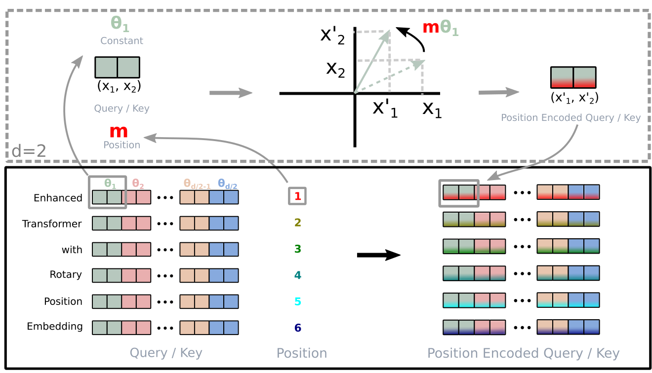
Split an even-dimensional vector into coordinate pairs and use a block-diagonal matrix of two-dimensional rotations, with geometrically spaced frequencies. Orthogonality preserves norms and gives RₘᵀRₙ=Rₙ₋ₘ, making the attention score relative. Figure 1 shows the operation. Equation 16’s final expanded expression has inconsistent token/projection-transpose notation; its original formula remains unchanged, while the preceding rotated-inner-product equality supplies the intended construction.

Equations 14–16
f{q,k}​(𝒙m,m)=𝑹Θ,md​𝑾{q,k}​𝒙mf_{\{q,k\}}({\boldsymbol{x}}_{m},m)={\boldsymbol{R}}^{d}_{\Theta,m}{\boldsymbol{W}}_{\{q,k\}}{\boldsymbol{x}}_{m} (14)
𝑹Θ,md=(cos⁡m​θ1−sin⁡m​θ100⋯00sin⁡m​θ1cos⁡m​θ100⋯0000cos⁡m​θ2−sin⁡m​θ2⋯0000sin⁡m​θ2cos⁡m​θ2⋯00⋱0000⋯cos⁡m​θd/2−sin⁡m​θd/20000⋯sin⁡m​θd/2cos⁡m​θd/2){\boldsymbol{R}}^{d}_{\Theta,m}=\begin{pmatrix}\cos{m\theta_{1}}&-\sin{m\theta_{1}}&0&0&\cdots&0&0\\ \sin{m\theta_{1}}&\cos{m\theta_{1}}&0&0&\cdots&0&0\\ 0&0&\cos{m\theta_{2}}&-\sin{m\theta_{2}}&\cdots&0&0\\ 0&0&\sin{m\theta_{2}}&\cos{m\theta_{2}}&\cdots&0&0\\ \vdots&\vdots&\vdots&\vdots&\ddots&\vdots&\vdots\\ 0&0&0&0&\cdots&\cos{m\theta_{d/2}}&-\sin{m\theta_{d/2}}\\ 0&0&0&0&\cdots&\sin{m\theta_{d/2}}&\cos{m\theta_{d/2}}\end{pmatrix} (15)
𝒒m⊺​𝒌n=(𝑹Θ,md​𝑾q​𝒙m)⊺​(𝑹Θ,nd​𝑾k​𝒙n)=𝒙⊺​𝑾q​RΘ,n−md​𝑾k​𝒙n{\boldsymbol{q}}_{m}^{\intercal}{\boldsymbol{k}}_{n}=({\boldsymbol{R}}^{d}_{\Theta,m}{\boldsymbol{W}}_{q}{\boldsymbol{x}}_{m})^{\intercal}({\boldsymbol{R}}^{d}_{\Theta,n}{\boldsymbol{W}}_{k}{\boldsymbol{x}}_{n})={\boldsymbol{x}}^{\intercal}{\boldsymbol{W}}_{q}R^{d}_{\Theta,n-m}{\boldsymbol{W}}_{k}{\boldsymbol{x}}_{n} (16)
Complete original Figure 1: Implementation of Rotary Position Embedding(RoPE).
Figure 1: Implementation of Rotary Position Embedding(RoPE).

3.3 Properties of RoPE

Two properties are examined: a distance-dependent bound induced by the frequency schedule, and a rotation-based extension of linear attention.

Long-term decay:

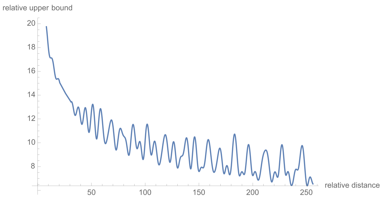
The chosen geometric frequencies produce the oscillatory upper-envelope behavior analyzed in §3.4.3. This supports a form of long-distance attenuation; it does not mean that every content-dependent attention score decreases monotonically as tokens move apart.

RoPE with linear attention:

Linear attention reassociates sums over feature-mapped keys and values to avoid a full pairwise attention matrix. RoPE rotates these query/key features in the numerator while leaving the normalization denominator unrotated. The paper does this to avoid introducing zero denominators through rotation. Numerator contributions can become negative, so this variant is not a probability distribution over values; it retains the associative computational structure.

Equations 17–19
Attention⁡(𝐐,𝐊,𝐕)m=∑n=1Nsim⁡(𝒒m,𝒌n)​𝒗n∑n=1Nsim⁡(𝒒m,𝒌n).\operatorname{Attention}(\mathbf{Q},\mathbf{K},\mathbf{V})_{m}=\frac{\sum_{n=1}^{N}\operatorname{sim}({\boldsymbol{q}}_{m},{\boldsymbol{k}}_{n}){\boldsymbol{v}}_{n}}{\sum_{n=1}^{N}\operatorname{sim}({\boldsymbol{q}}_{m},{\boldsymbol{k}}_{n})}. (17)
Attention⁡(𝑸,𝑲,𝑽)m=∑n=1Nϕ​(𝒒m)⊺​φ​(𝒌n)​𝒗n∑n=1Nϕ​(𝒒m)⊺​φ​(𝒌n),\operatorname{Attention}({\boldsymbol{Q}},{\boldsymbol{K}},{\boldsymbol{V}})_{m}=\frac{\sum_{n=1}^{N}\phi({\boldsymbol{q}}_{m})^{\intercal}\varphi({\boldsymbol{k}}_{n}){\boldsymbol{v}}_{n}}{\sum_{n=1}^{N}\phi({\boldsymbol{q}}_{m})^{\intercal}\varphi({\boldsymbol{k}}_{n})}, (18)
Attention⁡(𝐐,𝐊,𝐕)m=∑n=1N(𝑹Θ,md​ϕ​(𝒒m))⊺​(𝑹Θ,nd​φ​(𝒌n))​𝒗n∑n=1Nϕ​(𝒒m)⊺​φ​(𝒌n).\operatorname{Attention}(\mathbf{Q},\mathbf{K},\mathbf{V})_{m}=\frac{\sum_{n=1}^{N}\big({\boldsymbol{R}}^{d}_{\Theta,m}\phi({\boldsymbol{q}}_{m})\big)^{\intercal}\big({\boldsymbol{R}}^{d}_{\Theta,n}\varphi({\boldsymbol{k}}_{n})\big){\boldsymbol{v}}_{n}}{\sum_{n=1}^{N}\phi({\boldsymbol{q}}_{m})^{\intercal}\varphi({\boldsymbol{k}}_{n})}. (19)

3.4 Theoretical Explanation

The theory derives one family of valid two-dimensional maps, explains an elementwise implementation, and bounds the relative-position inner product using sums of complex phases.

3.4.1 Derivation of RoPE under 2D

Write query/key maps in polar form and impose their zero-position values and relative inner-product condition. A position-independent radius and content-independent relative phase lead to constant phase increments, hence a phase linear in position. Choosing linear token projections and zero common phase yields RoPE. This derives a particular solution rather than uniqueness among all encodings. Equations 20–33 are retained verbatim; the source’s exponential notation in Equation 31 and query-token index in Equation 32 contain apparent typesetting inconsistencies.

Equations 20–33
𝒒m\displaystyle{\boldsymbol{q}}_{m} =fq​(𝒙q,m),\displaystyle=f_{q}({\boldsymbol{x}}_{q},m), (20)
𝒌n\displaystyle{\boldsymbol{k}}_{n} =fk​(𝒙k,n),\displaystyle=f_{k}({\boldsymbol{x}}_{k},n),
𝒒m⊺​𝒌n=⟨fq​(𝒙m,m),fk​(𝒙n,n)⟩=g⁡(𝒙m,𝒙n,n−m),{\boldsymbol{q}}^{\intercal}_{m}{\boldsymbol{k}}_{n}=\langle f_{q}({\boldsymbol{x}}_{m},m),f_{k}({\boldsymbol{x}}_{n},n)\rangle=g({\boldsymbol{x}}_{m},{\boldsymbol{x}}_{n},n-m), (21)
𝒒\displaystyle{\boldsymbol{q}} =fq​(𝒙q,0),\displaystyle=f_{q}({\boldsymbol{x}}_{q},0), (22)
𝒌\displaystyle{\boldsymbol{k}} =fk​(𝒙k,0),\displaystyle=f_{k}({\boldsymbol{x}}_{k},0),
fq​(𝒙q,m)\displaystyle f_{q}({\boldsymbol{x}}_{q},m) =Rq​(𝒙q,m)​ei​Θq​(𝒙q,m),\displaystyle=R_{q}({\boldsymbol{x}}_{q},m)e^{i\Theta_{q}({\boldsymbol{x}}_{q},m)}, (23)
fk​(𝒙k,n)\displaystyle f_{k}({\boldsymbol{x}}_{k},n) =Rk​(𝒙k,n)​ei​Θk​(𝒙k,n),\displaystyle=R_{k}({\boldsymbol{x}}_{k},n)e^{i\Theta_{k}({\boldsymbol{x}}_{k},n)},
g⁡(𝒙q,𝒙k,n−m)\displaystyle g({\boldsymbol{x}}_{q},{\boldsymbol{x}}_{k},n-m) =Rg​(𝒙q,𝒙k,n−m)​ei​Θg​(𝒙q,𝒙k,n−m),\displaystyle=R_{g}({\boldsymbol{x}}_{q},{\boldsymbol{x}}_{k},n-m)e^{i\Theta_{g}({\boldsymbol{x}}_{q},{\boldsymbol{x}}_{k},n-m)},
Rq​(𝒙q,m)​Rk​(𝒙k,n)\displaystyle R_{q}({\boldsymbol{x}}_{q},m)R_{k}({\boldsymbol{x}}_{k},n) =Rg​(𝒙q,𝒙k,n−m),\displaystyle=R_{g}({\boldsymbol{x}}_{q},{\boldsymbol{x}}_{k},n-m), (24)
Θk​(𝒙k,n)−Θq​(𝒙q,m)\displaystyle\Theta_{k}({\boldsymbol{x}}_{k},n)-\Theta_{q}({\boldsymbol{x}}_{q},m) =Θg​(𝒙q,𝒙k,n−m),\displaystyle=\Theta_{g}({\boldsymbol{x}}_{q},{\boldsymbol{x}}_{k},n-m),
𝒒\displaystyle{\boldsymbol{q}} =‖𝒒‖​ei​θq=Rq​(𝒙q,0)​ei​Θq​(𝒙q,0),\displaystyle=\|{\boldsymbol{q}}\|e^{i\theta_{q}}=R_{q}({\boldsymbol{x}}_{q},0)e^{i\Theta_{q}({\boldsymbol{x}}_{q},0)}, (25)
𝒌\displaystyle{\boldsymbol{k}} =‖𝒌‖​ei​θk=Rk​(𝒙k,0)​ei​Θk​(𝒙k,0),\displaystyle=\|{\boldsymbol{k}}\|e^{i\theta_{k}}=R_{k}({\boldsymbol{x}}_{k},0)e^{i\Theta_{k}({\boldsymbol{x}}_{k},0)},
Rq​(𝒙q,m)​Rk​(𝒙k,m)\displaystyle R_{q}({\boldsymbol{x}}_{q},m)R_{k}({\boldsymbol{x}}_{k},m) =Rg​(𝒙q,𝒙k,0)=Rq​(𝒙q,0)​Rk​(𝒙k,0)=‖𝒒‖​‖𝒌‖,\displaystyle=R_{g}({\boldsymbol{x}}_{q},{\boldsymbol{x}}_{k},0)=R_{q}({\boldsymbol{x}}_{q},0)R_{k}({\boldsymbol{x}}_{k},0)=\|{\boldsymbol{q}}\|\|{\boldsymbol{k}}\|, (26a)
Θk​(𝒙k,m)−Θq​(𝒙q,m)\displaystyle\Theta_{k}({\boldsymbol{x}}_{k},m)-\Theta_{q}({\boldsymbol{x}}_{q},m) =Θg​(𝒙q,𝒙k,0)=Θk​(𝒙k,0)−Θq​(𝒙q,0)=θk−θq.\displaystyle=\Theta_{g}({\boldsymbol{x}}_{q},{\boldsymbol{x}}_{k},0)=\Theta_{k}({\boldsymbol{x}}_{k},0)-\Theta_{q}({\boldsymbol{x}}_{q},0)=\theta_{k}-\theta_{q}. (26b)
Rq​(𝒙q,m)\displaystyle R_{q}({\boldsymbol{x}}_{q},m) =Rq​(𝒙q,0)=‖𝒒‖\displaystyle=R_{q}({\boldsymbol{x}}_{q},0)=\|{\boldsymbol{q}}\| (27)
Rk​(𝒙k,n)\displaystyle R_{k}({\boldsymbol{x}}_{k},n) =Rk​(𝒙k,0)=‖𝒌‖\displaystyle=R_{k}({\boldsymbol{x}}_{k},0)=\|{\boldsymbol{k}}\|
Rg​(𝒙q,𝒙k,n−m)\displaystyle R_{g}({\boldsymbol{x}}_{q},{\boldsymbol{x}}_{k},n-m) =Rg​(𝒙q,𝒙k,0)=‖𝒒‖​‖𝒌‖\displaystyle=R_{g}({\boldsymbol{x}}_{q},{\boldsymbol{x}}_{k},0)=\|{\boldsymbol{q}}\|\|{\boldsymbol{k}}\|
Θf​(𝒙{q,k},m)=ϕ⁡(m)+θ{q,k},\Theta_{f}({\boldsymbol{x}}_{\{q,k\}},m)=\phi(m)+\theta_{\{q,k\}}, (28)
ϕ⁡(m+1)−ϕ⁡(m)=Θg​(𝒙q,𝒙k,1)+θq−θk,\phi(m+1)-\phi(m)=\Theta_{g}({\boldsymbol{x}}_{q},{\boldsymbol{x}}_{k},1)+\theta_{q}-\theta_{k}, (29)
ϕ⁡(m)=m​θ+γ,\phi(m)=m\theta+\gamma, (30)
fq​(𝒙q,m)\displaystyle f_{q}({\boldsymbol{x}}_{q},m) =‖𝒒‖​ei​θq+m​θ+γ=𝒒​ei⁡(m​θ+γ),\displaystyle=\|{\boldsymbol{q}}\|e^{i\theta_{q}+m\theta+\gamma}={\boldsymbol{q}}e^{i(m\theta+\gamma)}, (31)
fk​(𝒙k,n)\displaystyle f_{k}({\boldsymbol{x}}_{k},n) =‖𝒌‖​ei​θk+n​θ+γ=𝒌​ei⁡(n​θ+γ).\displaystyle=\|{\boldsymbol{k}}\|e^{i\theta_{k}+n\theta+\gamma}={\boldsymbol{k}}e^{i(n\theta+\gamma)}.
𝒒=fq​(𝒙m,0)\displaystyle{\boldsymbol{q}}=f_{q}({\boldsymbol{x}}_{m},0) =𝑾q​𝒙n,\displaystyle={\boldsymbol{W}}_{q}{\boldsymbol{x}}_{n}, (32)
𝒌=fk​(𝒙n,0)\displaystyle{\boldsymbol{k}}=f_{k}({\boldsymbol{x}}_{n},0) =𝑾k​𝒙n.\displaystyle={\boldsymbol{W}}_{k}{\boldsymbol{x}}_{n}.
fq​(𝒙m,m)\displaystyle f_{q}({\boldsymbol{x}}_{m},m) =(𝑾q​𝒙m)​ei​m​θ,\displaystyle=({\boldsymbol{W}}_{q}{\boldsymbol{x}}_{m})e^{im\theta}, (33)
fk​(𝒙n,n)\displaystyle f_{k}({\boldsymbol{x}}_{n},n) =(𝑾k​𝒙n)​ei​n​θ.\displaystyle=({\boldsymbol{W}}_{k}{\boldsymbol{x}}_{n})e^{in\theta}.

3.4.2 Computational efficient realization of rotary matrix multiplication

A dense rotation matrix is unnecessary. Multiply the original coordinates by cosines and a signed, pair-swapped vector by sines, then add them. Equation 34 exposes this elementwise implementation and preserves the pairwise rotation exactly.

Equation 34
𝑹Θ,md​𝒙=(x1x2x3x4xd−1xd)⊗(cos⁡m​θ1cos⁡m​θ1cos⁡m​θ2cos⁡m​θ2cos⁡m​θd/2cos⁡m​θd/2)+(−x2x1−x4x3−xdxd−1)⊗(sin⁡m​θ1sin⁡m​θ1sin⁡m​θ2sin⁡m​θ2sin⁡m​θd/2sin⁡m​θd/2){\boldsymbol{R}}^{d}_{\Theta,m}{\boldsymbol{x}}=\begin{pmatrix}x_{1}\\ x_{2}\\ x_{3}\\ x_{4}\\ \vdots\\ x_{d-1}\\ x_{d}\end{pmatrix}\otimes\begin{pmatrix}\cos{m\theta_{1}}\\ \cos{m\theta_{1}}\\ \cos{m\theta_{2}}\\ \cos{m\theta_{2}}\\ \vdots\\ \cos{m\theta_{d/2}}\\ \cos{m\theta_{d/2}}\end{pmatrix}+\begin{pmatrix}-x_{2}\\ x_{1}\\ -x_{4}\\ x_{3}\\ \vdots\\ -x_{d}\\ x_{d-1}\end{pmatrix}\otimes\begin{pmatrix}\sin{m\theta_{1}}\\ \sin{m\theta_{1}}\\ \sin{m\theta_{2}}\\ \sin{m\theta_{2}}\\ \vdots\\ \sin{m\theta_{d/2}}\\ \sin{m\theta_{d/2}}\end{pmatrix} (34)

3.4.3 Long-term decay of RoPE

Express the score as a real part of a sum of complex coordinate-pair products. Abel transformation bounds it by a content-dependent adjacent-product variation term times a sum of partial phase sums. Figure 2 plots the oscillatory relative-distance bound for the selected frequency schedule. The argument concerns this bound, not a general guarantee of context-length generalization or strictly monotone attention weights.

Equations 35–37
(𝑹Θ,md𝑾q𝒙m)⊺(𝑹Θ,nd𝑾k𝒙n)=Re[∑i=0d/2−1𝒒[2i:2i+1]𝒌[2i:2i+1]∗ei⁡(m−n)​θi]({\boldsymbol{R}}^{d}_{\Theta,m}{\boldsymbol{W}}_{q}{\boldsymbol{x}}_{m})^{\intercal}({\boldsymbol{R}}^{d}_{\Theta,n}{\boldsymbol{W}}_{k}{\boldsymbol{x}}_{n})=\operatorname{Re}\bigg[\sum_{i=0}^{d/2-1}{\boldsymbol{q}}_{[2i:2i+1]}{\boldsymbol{k}}_{[2i:2i+1]}^{*}e^{i(m-n)\theta_{i}}\bigg] (35)
∑i=0d/2−1𝒒[2i:2i+1]𝒌[2i:2i+1]∗ei⁡(m−n)​θi=∑i=0d/2−1hi(Si+1−Si)=−∑i=0d/2−1Si+1(hi+1−hi).\sum_{i=0}^{d/2-1}{\boldsymbol{q}}_{[2i:2i+1]}{\boldsymbol{k}}_{[2i:2i+1]}^{*}e^{i(m-n)\theta_{i}}=\sum_{i=0}^{d/2-1}h_{i}(S_{i+1}-S_{i})=-\sum_{i=0}^{d/2-1}S_{i+1}(h_{i+1}-h_{i}). (36)
|∑i=0d/2−1𝒒[2i:2i+1]𝒌[2i:2i+1]∗ei⁡(m−n)​θi|\displaystyle\bigg|\sum_{i=0}^{d/2-1}{\boldsymbol{q}}_{[2i:2i+1]}{\boldsymbol{k}}_{[2i:2i+1]}^{*}e^{i(m-n)\theta_{i}}\bigg| =|∑i=0d/2−1Si+1​(hi+1−hi)|\displaystyle=\bigg|\sum_{i=0}^{d/2-1}S_{i+1}(h_{i+1}-h_{i})\bigg| (37)
≤∑i=0d/2−1|Si+1|​|(hi+1−hi)|\displaystyle\leq\sum_{i=0}^{d/2-1}|S_{i+1}||(h_{i+1}-{h_{i}})|
≤(maxi⁡|hi+1−hi|)​∑i=0d/2−1|Si+1|\displaystyle\leq\big(\max_{i}|h_{i+1}-h_{i}|\big)\sum_{i=0}^{d/2-1}|S_{i+1}|
Complete original Figure 2: Long-term decay of RoPE.
Figure 2: Long-term decay of RoPE.

4 Experiments and Evaluation

Experiments cover translation, English masked-language pretraining, GLUE, Performer language modeling and Chinese long-document matching. The tasks test different implementations and protocols; their results should be interpreted separately.

4.1 Machine Translation

Translation compares a Transformer baseline with the corresponding rotary-position variant on WMT 2014 English–German.

4.1.1 Experimental Settings

The dataset contains approximately 4.5 million parallel sentence pairs. The baseline follows the Transformer setup.

4.1.2 Implementation details

Use a joint 37,000-token byte-pair vocabulary, average the final five checkpoints, and decode with beam size four and length penalty .6. Fairseq training uses Adam with betas (.9,.98), learning-rate warmup from 10⁻⁷ to 5×10⁻⁴ followed by inverse-square-root decay, and label smoothing .1. Report BLEU.

4.1.3 Results

Table 1 reports BLEU 27.5 for RoFormer versus 27.3 for Transformer-base under the stated common setup: a modest .2-point improvement.

Table 1: The proposed RoFormer gives better BLEU scores compared to its baseline alternative Vaswani et al. (2017) on the WMT 2014 English-to-German translation taskBojar et al. (2014).
Model BLEU
Transformer-baseVaswani et al. (2017) 27.3
RoFormer 27.5

4.2 Pre-training Language Modeling

English pretraining compares a BERT-based model with a rotary variant. The source calls BERT’s replaced position encoding “sinusoidal”; this is the paper’s implementation description, not a property of standard learned-position BERT.

4.2.1 Experimental Settings

BookCorpus and English Wikipedia are split 80:20 for training and validation. Masked-language-modeling loss is the metric, and bert-base-uncased supplies the baseline configuration.

4.2.2 Implementation details

The stated protocol trains for 100,000 steps with batch size 64, maximum length 512 and AdamW learning rate 10⁻⁵. Rotary query/key attention follows Equation 16.

4.2.3 Results

Figure 3’s left panel shows faster training-loss reduction for RoFormer. This plot is evidence about optimization under the reported setup, not by itself a held-out generalization or wall-clock efficiency result.
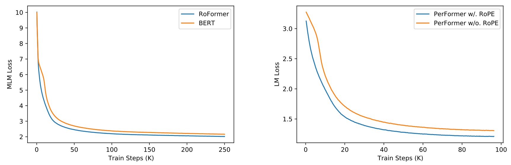
Complete original Figure 3: Evaluation of RoPE in language modeling pre-training. Left : training loss for BERT and RoFormer. Right : training loss for PerFormer with and without RoPE.
Figure 3: Evaluation of RoPE in language modeling pre-training. Left: training loss for BERT and RoFormer. Right: training loss for PerFormer with and without RoPE.

4.3 Fine-tuning on GLUE tasks

GLUE fine-tuning tests whether pretrained rotary representations transfer across six language-understanding tasks.

4.3.1 Experimental Settings

Report F1 for MRPC and QQP, Spearman correlation for STS-B, and accuracy for SST-2, QNLI and the matched/mismatched MNLI sets. The tasks use different score definitions.

4.3.2 Implementation details

Fine-tune with the Transformers library for three epochs, maximum length 512 and batch size 32. Search learning rates 2, 3, 4 and 5×10⁻⁵, reporting the source’s best-averaged validation results. Table 2 preserves the complete comparison.

Table 2: Comparing RoFormer and BERT by fine tuning on downstream GLEU tasks.
Model MRPC SST-2 QNLI STS-B QQP MNLI(m/mm)
BERTDevlin et al. (2019) 88.9 93.5 90.5 85.8 71.2 84.6/83.4
RoFormer 89.5 90.7 88.0 87.0 86.4 80.2/79.8

4.3.3 Results

RoFormer improves MRPC (89.5 versus 88.9), STS-B (87.0 versus 85.8) and QQP (86.4 versus 71.2), but scores lower on SST-2, QNLI and both MNLI sets. Thus this table supports task-specific gains, not consistent superiority across GLUE.

4.4 Performer with RoPE

Performer provides a linear-attention test bed. Apply the rotary construction from §3.3 while retaining the reassociated attention computation.

4.4.1 Implementation details

Character-level Enwik8 modeling uses twelve layers, hidden width 768, twelve heads, learning rate 10⁻⁴, batch size 128 and fixed sequence length 1,024. The source identifies the Performer implementation.

4.4.2 Results

Figure 3’s right panel shows lower training loss with RoPE at the same training-step budget. It illustrates compatibility and an optimization benefit in this setup; it does not measure a complete runtime comparison.

4.5 Evaluation on Chinese Data

Chinese experiments evaluate document matching with texts commonly longer than 512 characters, using a word-tokenized rotary model and several pretrained baselines.

4.5.1 Implementation

Replace WoBERT’s absolute positions with RoPE. Table 3 distinguishes this word-level tokenizer from the character-level BERT and NEZHA baselines, alongside their position encodings. Tokenization is therefore an additional difference in some comparisons.

Table 3: Cross-comparison between our RoFormer and other pre-trained models on Chinese data. ’abs’ and ’rel’ annotates absolute position embedding and relative position embedding, respectively.
Model BERTDevlin et al. (2019) WoBERTSu (2020) NEZHAWei et al. (2019) RoFormer
Tokenization level char word char word
Position embedding abs. abs. rel. RoPE

4.5.2 Pre-training

Pretrain on approximately 34 GB of Chinese Wikipedia, news and forum text in six consecutive stages. Table 4 preserves each length, batch size, step count, loss and accuracy. Lengths range from 128 to 1,536. Because training continues while multiple settings change, differences between stages do not isolate a causal effect of context length.

Table 4: Pre-training strategy of RoFormer on Chinese dataset. The training procedure is divided into various consecutive stages. In each stage, we train the model with a specific combination of maximum sequence length and batch size.
Stage Max seq length Batch size Training steps Loss Accuracy
1 512 256 200k 1.73 65.0%
2 1536 256 12.5k 1.61 66.8%
3 256 256 120k 1.75 64.6%
4 128 512 80k 1.83 63.4%
5 1536 256 10k 1.58 67.4%
6 512 512 30k 1.66 66.2%

4.5.3 Downstream Tasks & Dataset

CAIL2019-SCM contains 8,964 triples of legal cases. Given (A,B,C), predict whether A is closer to B or C. Split the data 60:20:20 for training, validation and testing; documents are generally longer than 512 characters.

4.5.4 Results

At length 512, RoFormer’s test accuracy is 68.29%, versus WoBERT’s 68.10% and BERT’s 67.77%. RoFormer at 1,024 reaches 69.79%. The within-RoFormer improvement is 1.50 percentage points; the improvement over WoBERT-512 is 1.69 points. The source prose conflates these comparisons, so Table 5’s exact values are the basis here.

Table 5: Experiment results on CAIL2019-SCM task. Numbers in the first column denote the maximum cut-off sequence length. The results are presented in terms of percent accuracy.
Model Validation Test
BERT-512 64.13% 67.77%
WoBERT-512 64.07% 68.10%
RoFormer-512 64.13% 68.29%
RoFormer-1024 66.07% 69.79%

4.5.5 Limitations of the work

The authors do not fully explain why the rotary model converges faster or performs better on the long-text task. The distance analysis alone does not establish those empirical effects. Pretraining also requires substantial hardware resources.

5 Conclusions

RoPE supplies a norm-preserving positional transform whose query–key product depends on relative displacement, with an efficient coordinatewise implementation and a linear-attention variant. Selected experiments support its usefulness, while mixed downstream results, implementation differences and unresolved explanations limit broader claims.

Concept demonstration

Open image ↗