Overview
Cross-layer transcoders provide a sparse replacement model for investigating how language models compute particular responses.
Introduction
The method learns interpretable computational features, traces their interactions on individual prompts, and tests proposed mechanisms through interventions. Case studies cover acronym completion, factual recall, and addition; a companion report studies more complex behaviors. Following earlier transcoder work, the graphs describe a simplified replacement model rather than a complete causal explanation of the original transformer.
Building an Interpretable Replacement Model
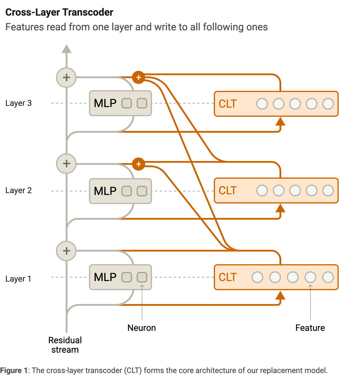
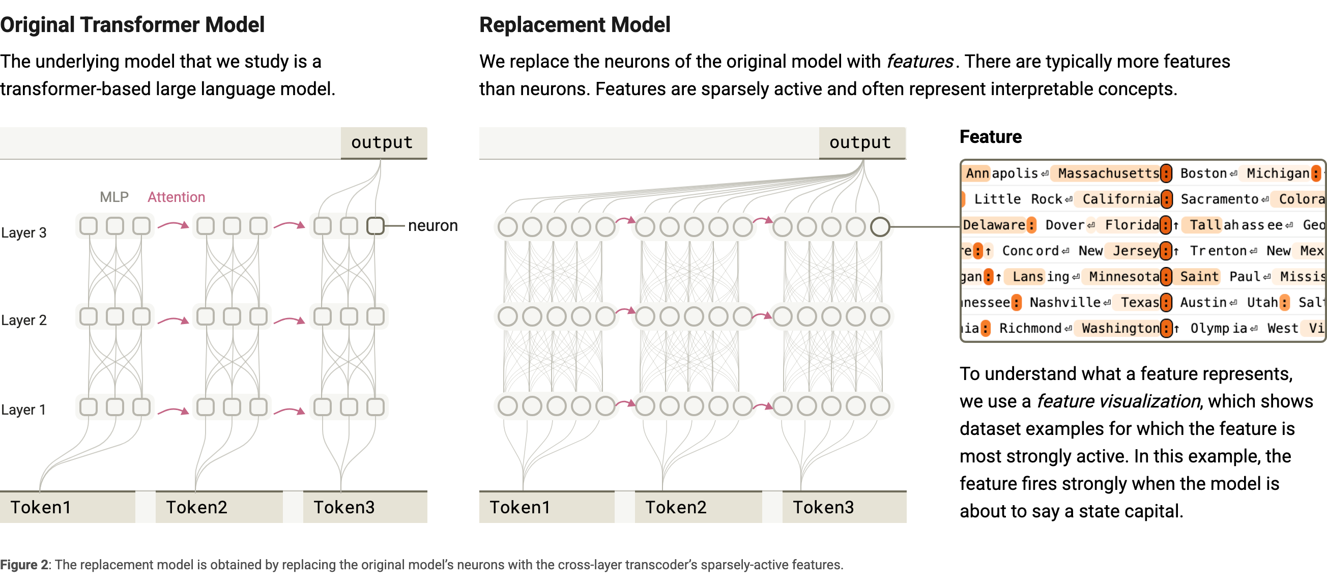
A replacement model approximates the transformer’s MLP computations with sparse learned features while retaining the original attention and residual pathways.
Architecture
Each CLT feature reads the residual stream at one layer, applies JumpReLU, and writes to that and later MLP outputs. Joint reconstruction and sparsity objectives encourage compact computational units that can absorb repeated cross-layer amplification. The experiments use an eighteen-layer research model and Claude 3.5 Haiku.
Equations
From Cross-Layer Transcoder to Replacement Model
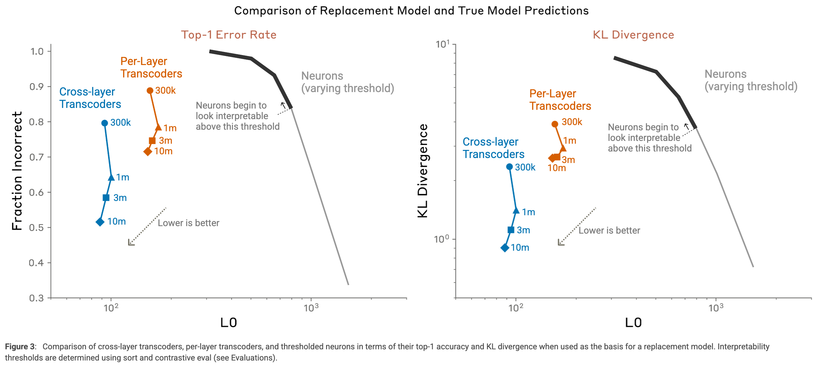
Running the replacement sequentially reproduces the original model’s next-token choice only about half the time in the largest eighteen-layer experiment, on a selected nontrivial prompt set. CLTs outperform comparable per-layer transcoders, but discrepancies compound across layers.
The Local Replacement Model
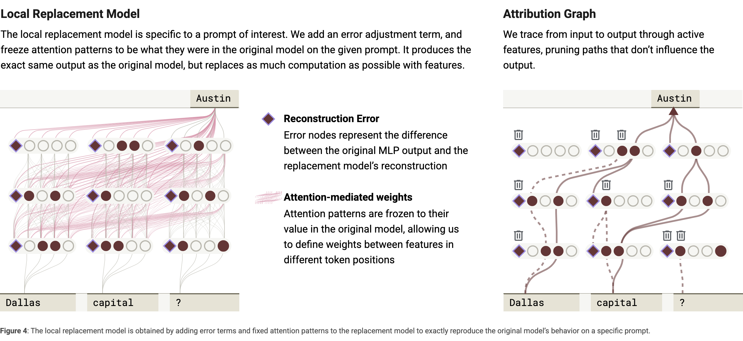
A prompt-specific local replacement model freezes attention patterns and normalization denominators and adds the original reconstruction errors as constants. It therefore exactly matches the unperturbed forward pass. This equality is guaranteed by construction and does not establish faithful behavior under interventions.
Attribution Graphs
Attribution graphs expose direct linear interactions between active features after the remaining nonlinear components are held fixed.
Constructing an Attribution Graph for a Prompt
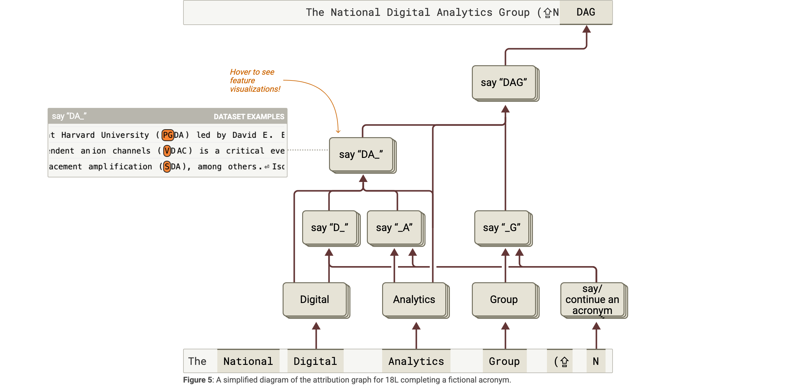
Nodes represent active features, input embeddings, reconstruction errors, and selected output logits. Edges combine source activation with a backward-Jacobian-derived virtual weight. They include information transported through frozen attention but omit why attention selected those positions. Influence-based pruning makes the graphs smaller while sacrificing some explanatory coverage.
Equation
Learning from Attribution Graphs
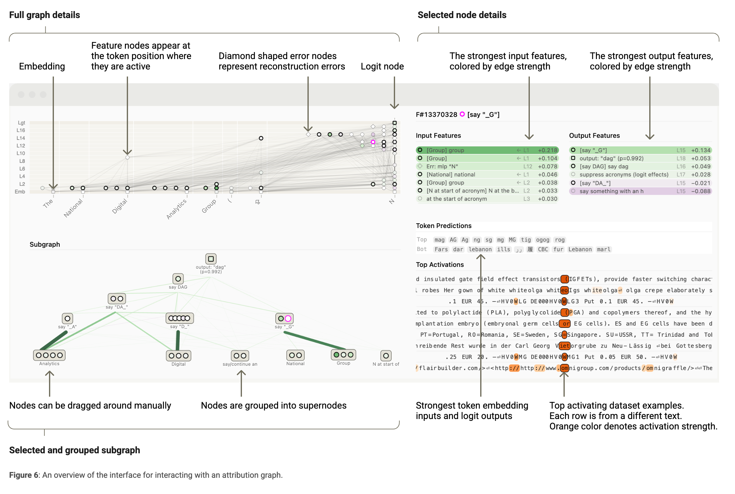
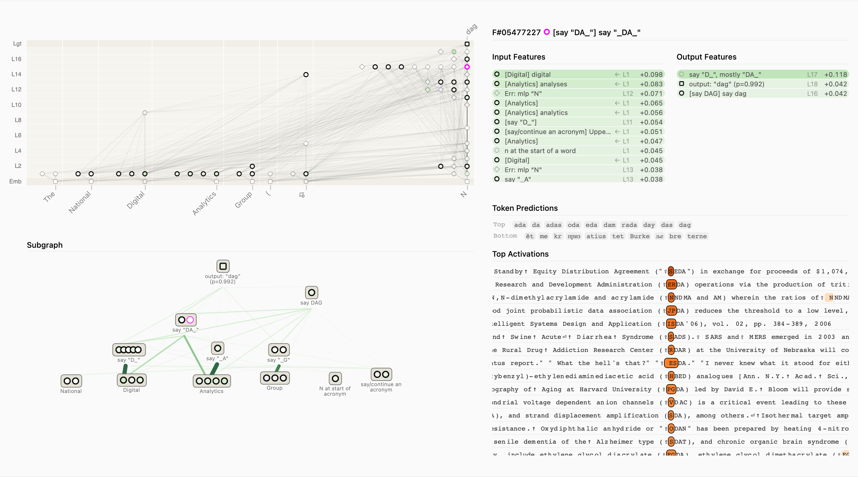
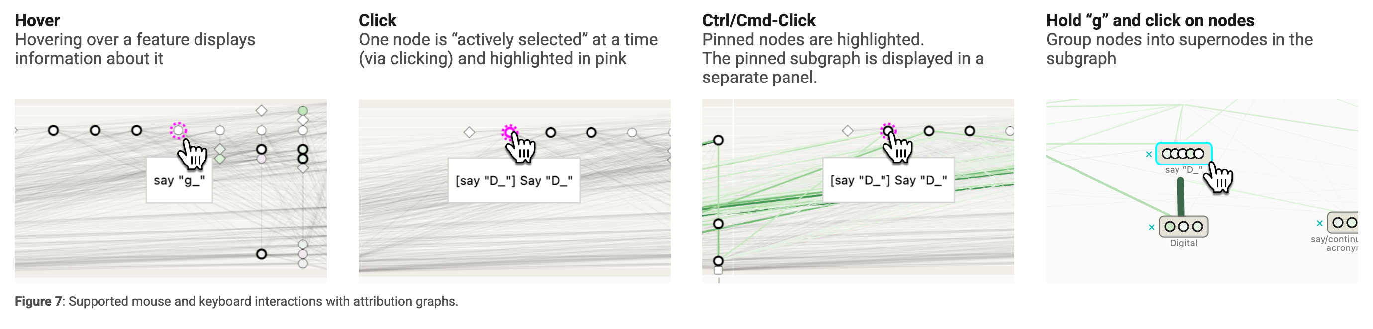
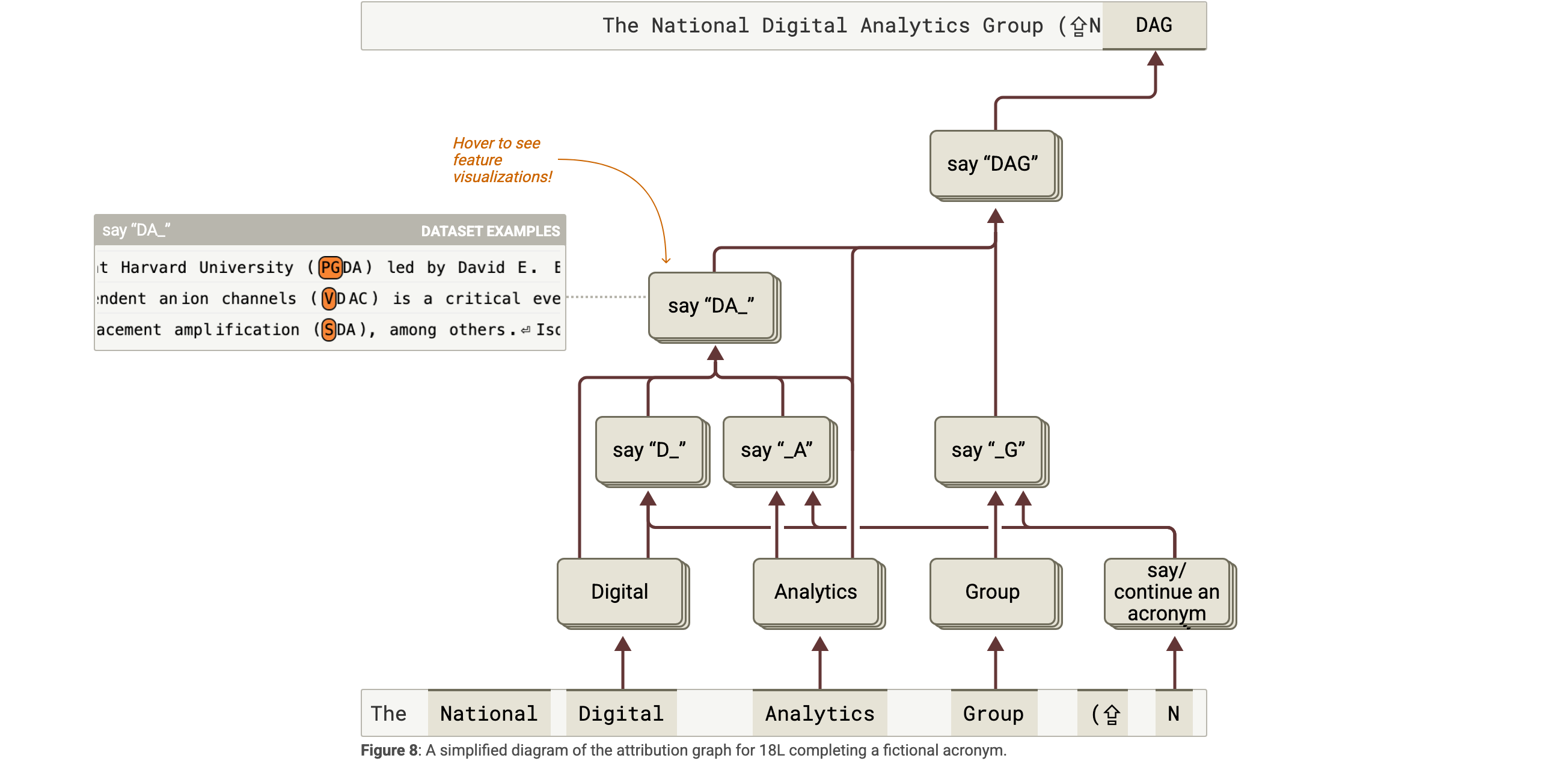
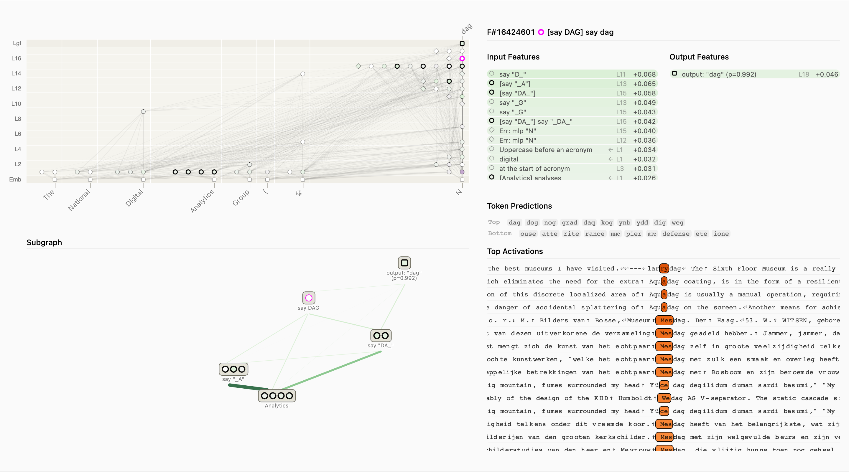
The acronym example follows National Digital Analytics Group to its acronym continuation. The original interface supports tracing, feature inspection, and manual grouping; the retained still images show its published state.
Understanding and Labeling Features
Feature labels combine activation examples, promoted or suppressed tokens, and neighboring features. Input and output features are often easier to name than intermediate abstractions. Polysemantic examples and context-dependent facets make labels provisional; even imperfect labels can reveal useful graph structure.
Grouping Features into Supernodes
Supernodes group features with a shared role on the current prompt, such as detecting a word’s initial. Grouping may depend on activation patterns, output effects, or connectivity. It is a subjective simplification, not an independently validated discovery of canonical components.
Validating Attribution Graph Hypotheses with Interventions
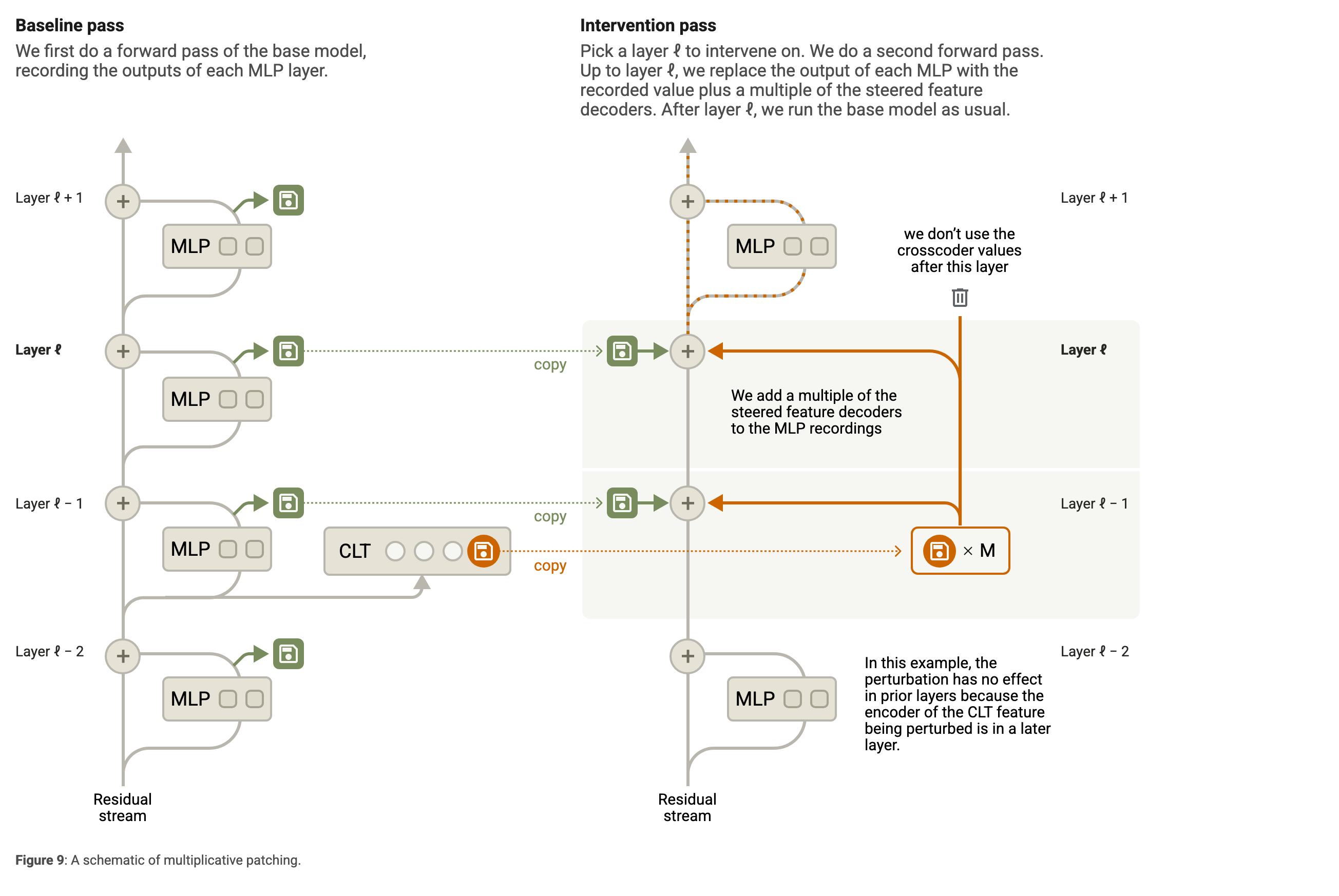
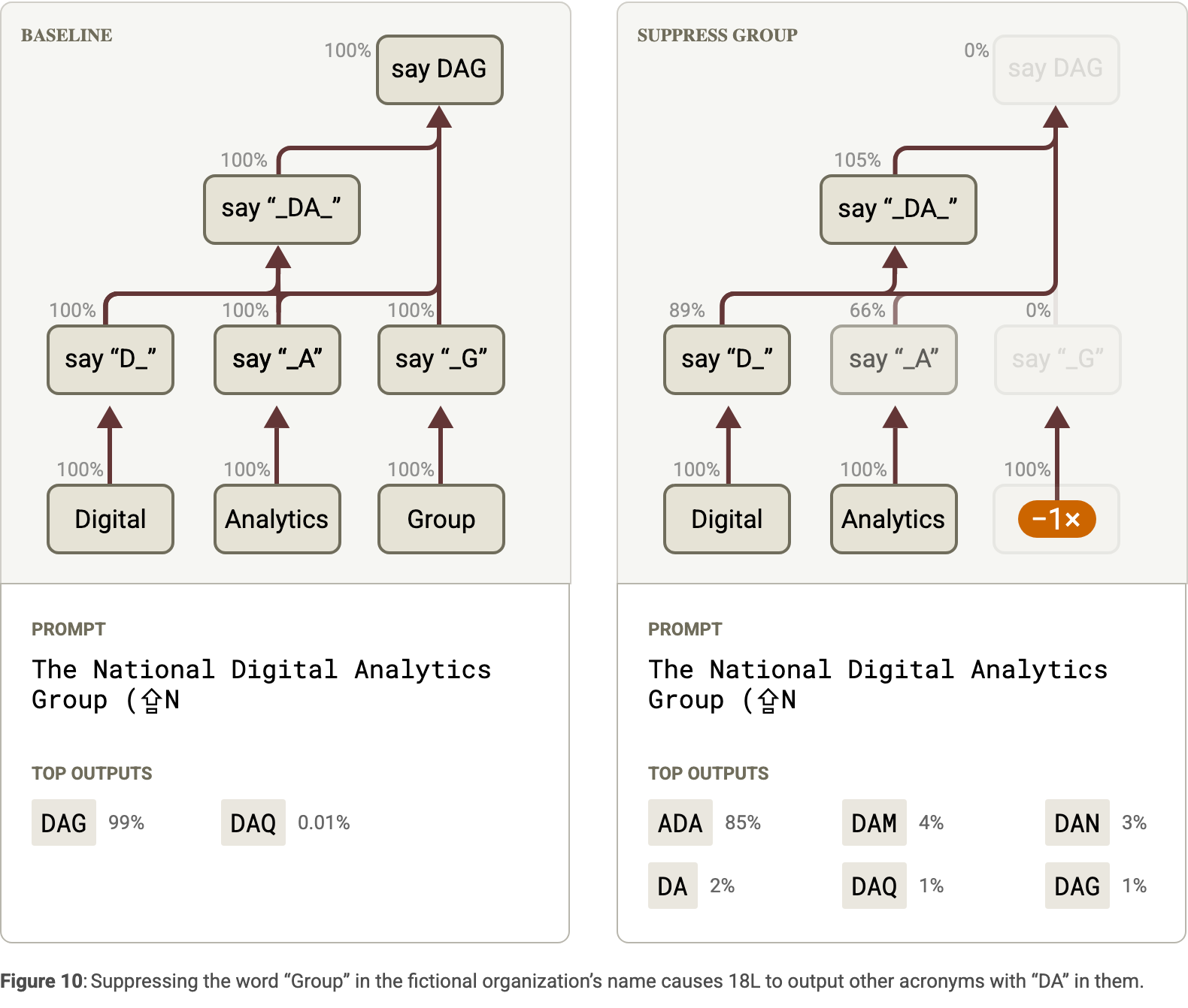
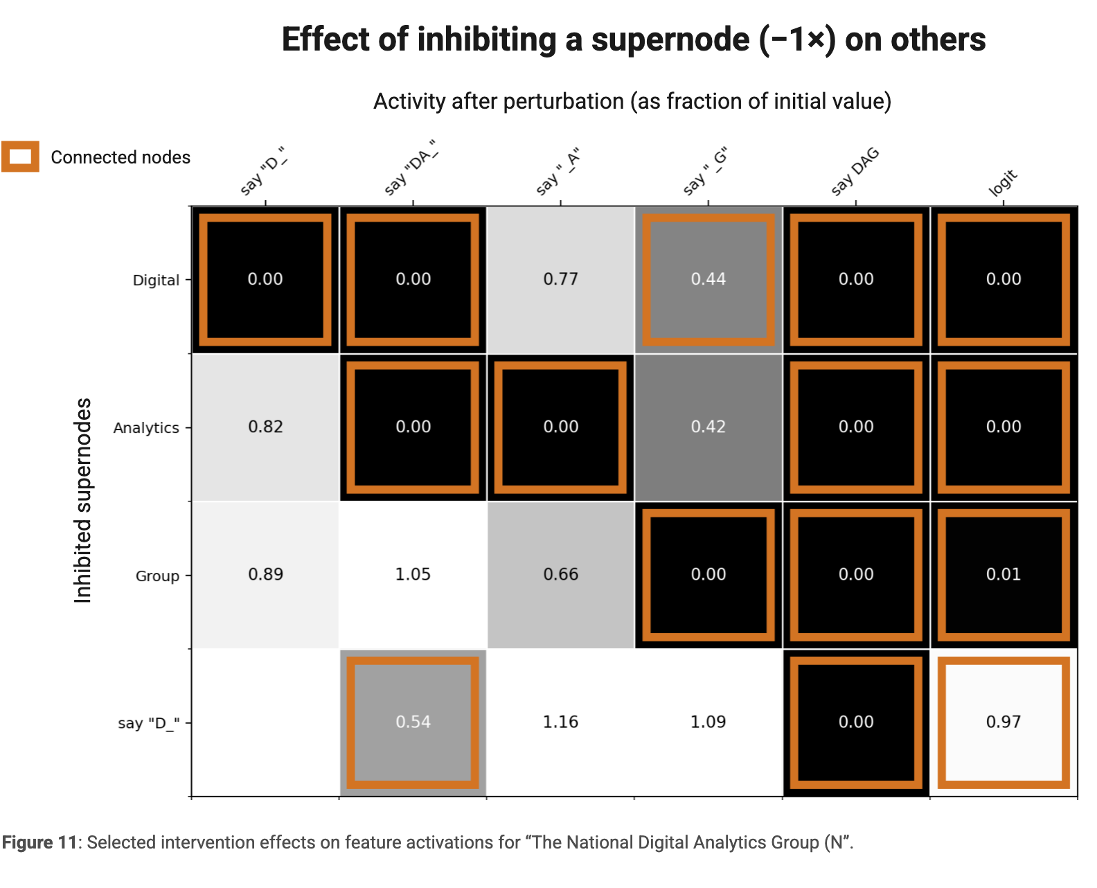
Constrained patching changes feature decodings across a chosen layer range while clamping intervening MLP outputs. The model then continues from that range, with attention fixed. Acronym interventions support predicted word-to-initial-to-output dependencies, but direct effects within the patching range are partly guaranteed by the method.
Localizing Important Layers
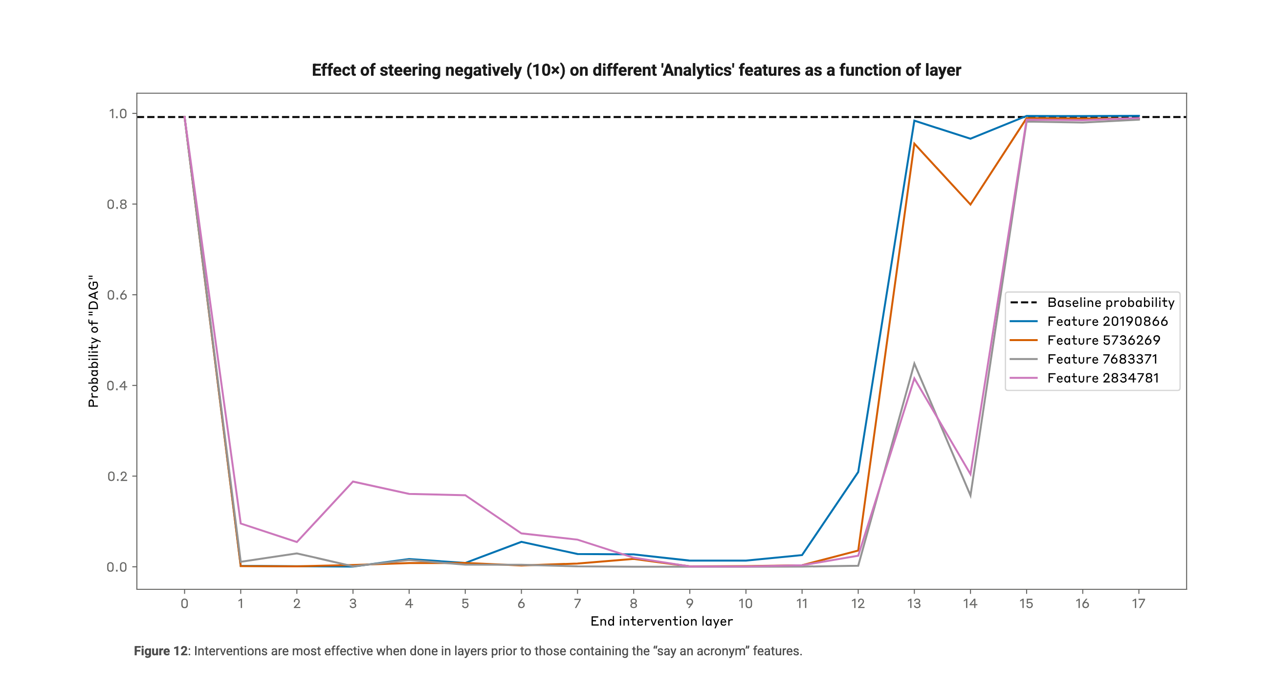
Sweeping the final patching layer localizes where a feature matters. The Analytics example loses influence once patching overwrites downstream mediators, illustrating why layer choice changes the interpretation of an intervention.
Factual Recall Case Study
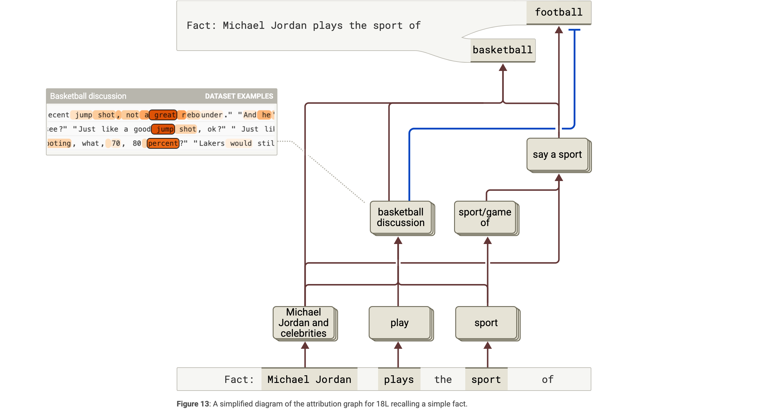
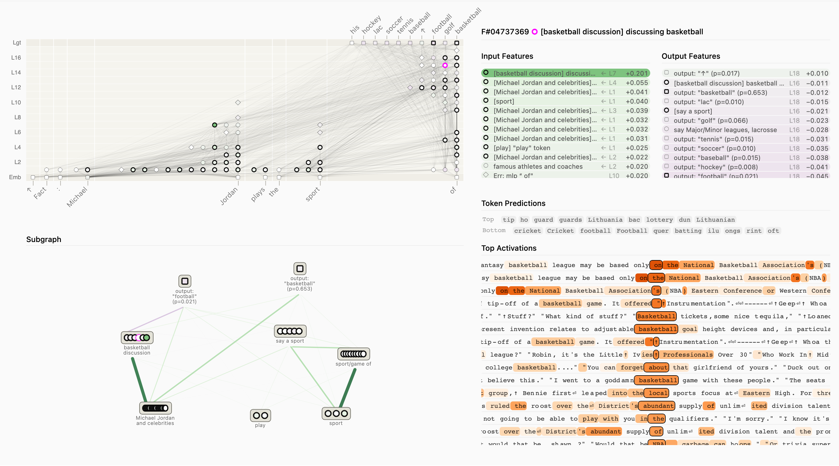
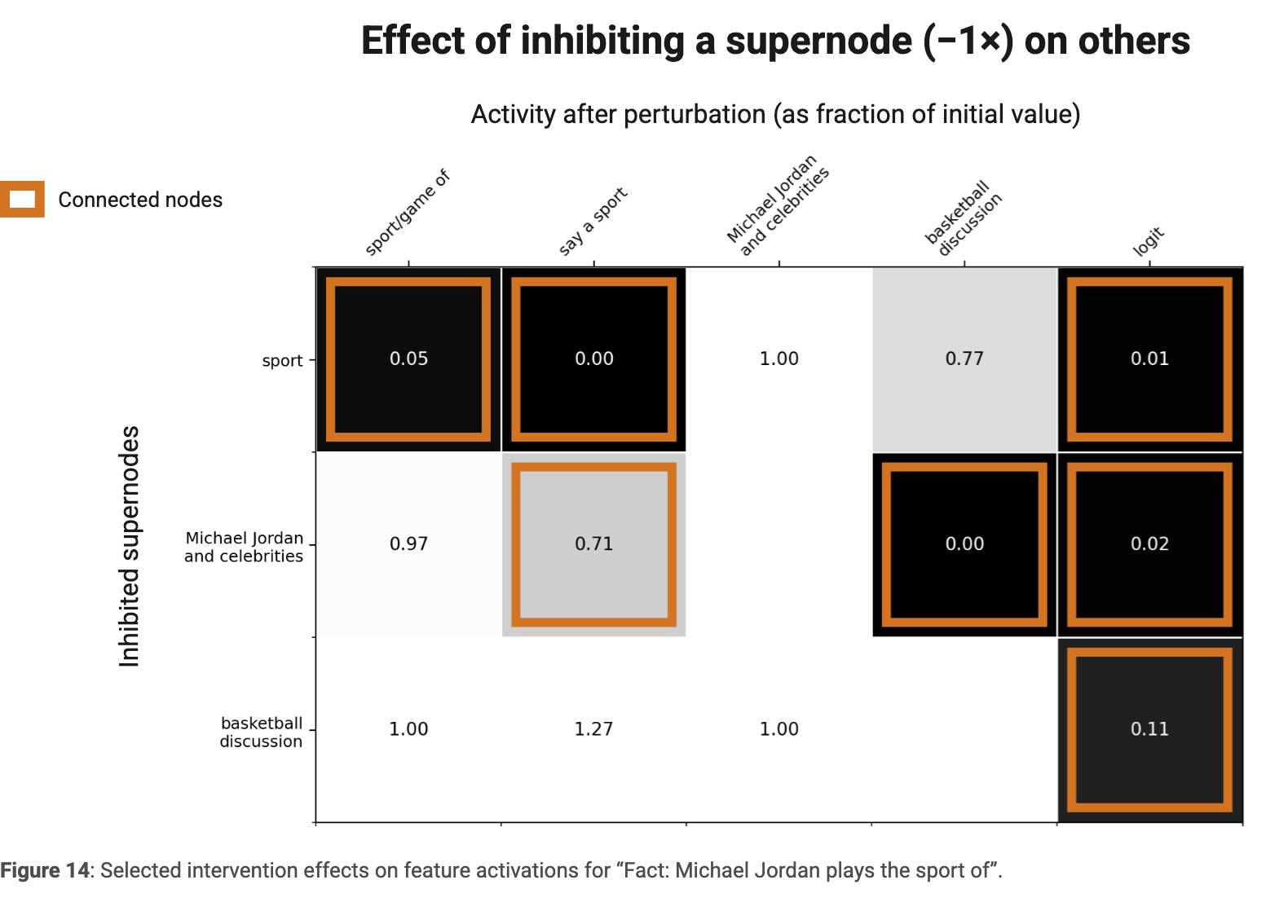
Michael Jordan→basketball recall combines an entity-specific path with a generic request-for-a-sport path, plus direct shortcuts. Suppressing the entity and sport supernodes mostly affects their own branches; inhibiting intermediate basketball features also changes the output. Some grouped features remain polysemantic.
Addition Case Study
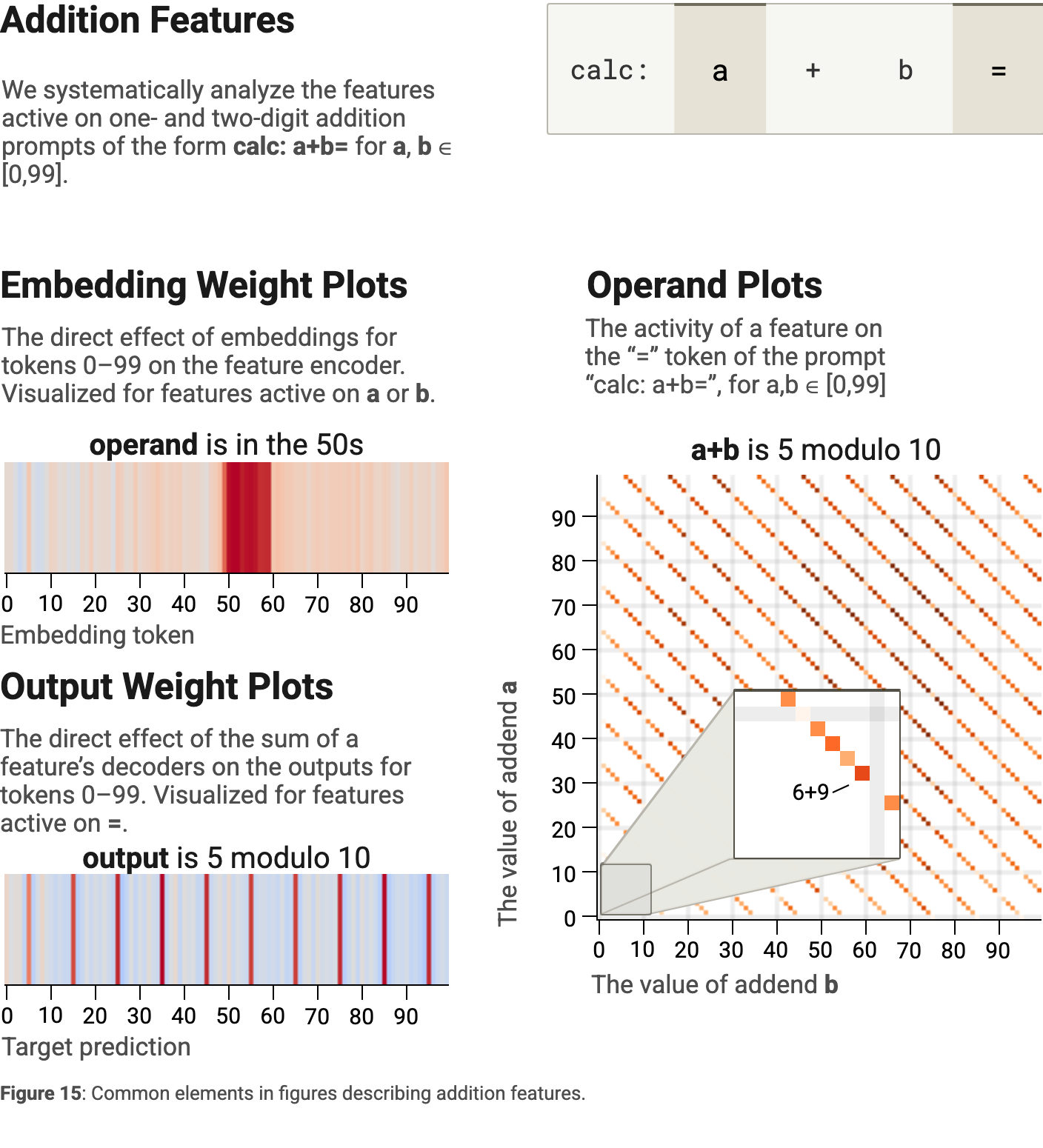
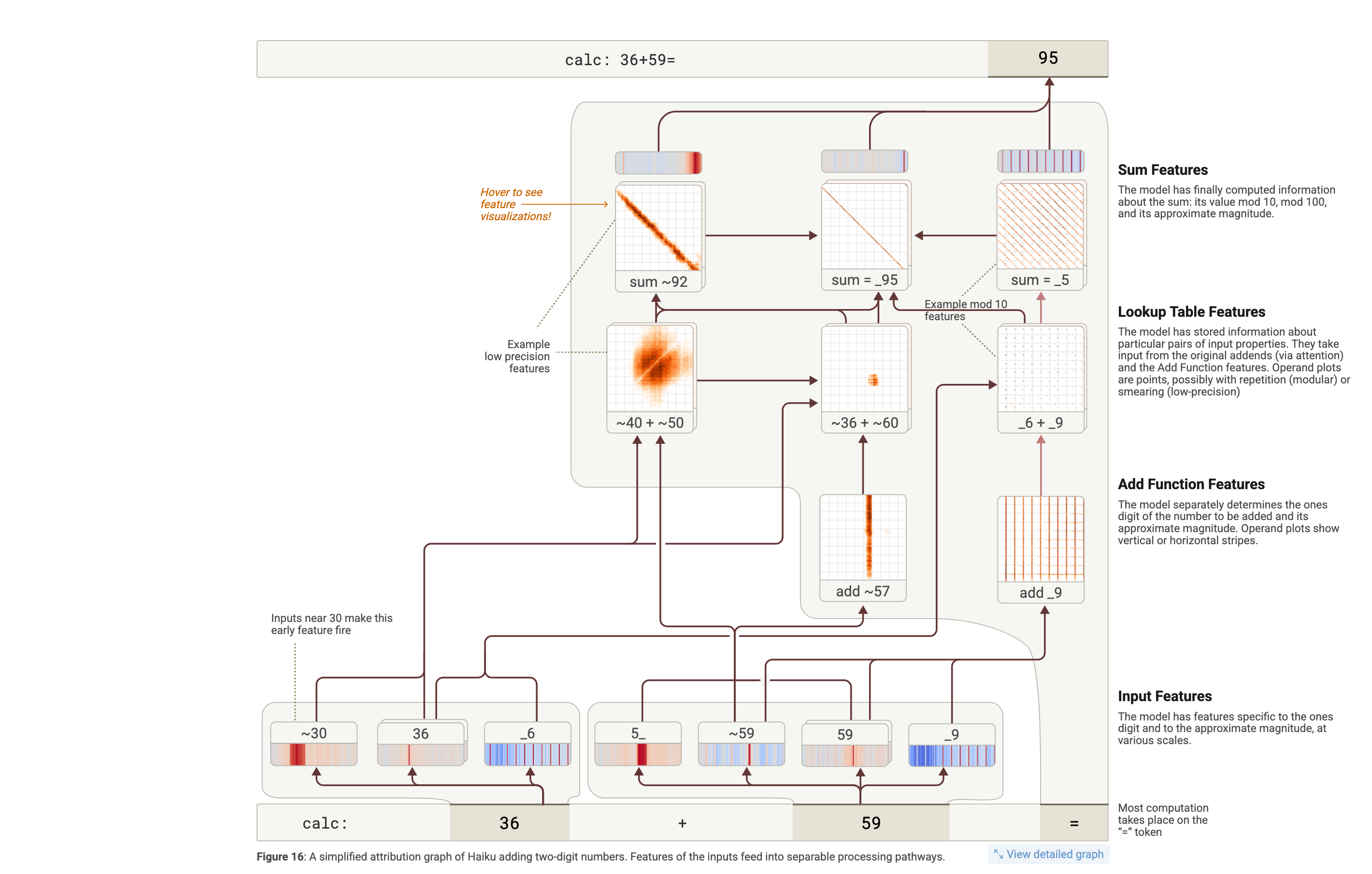
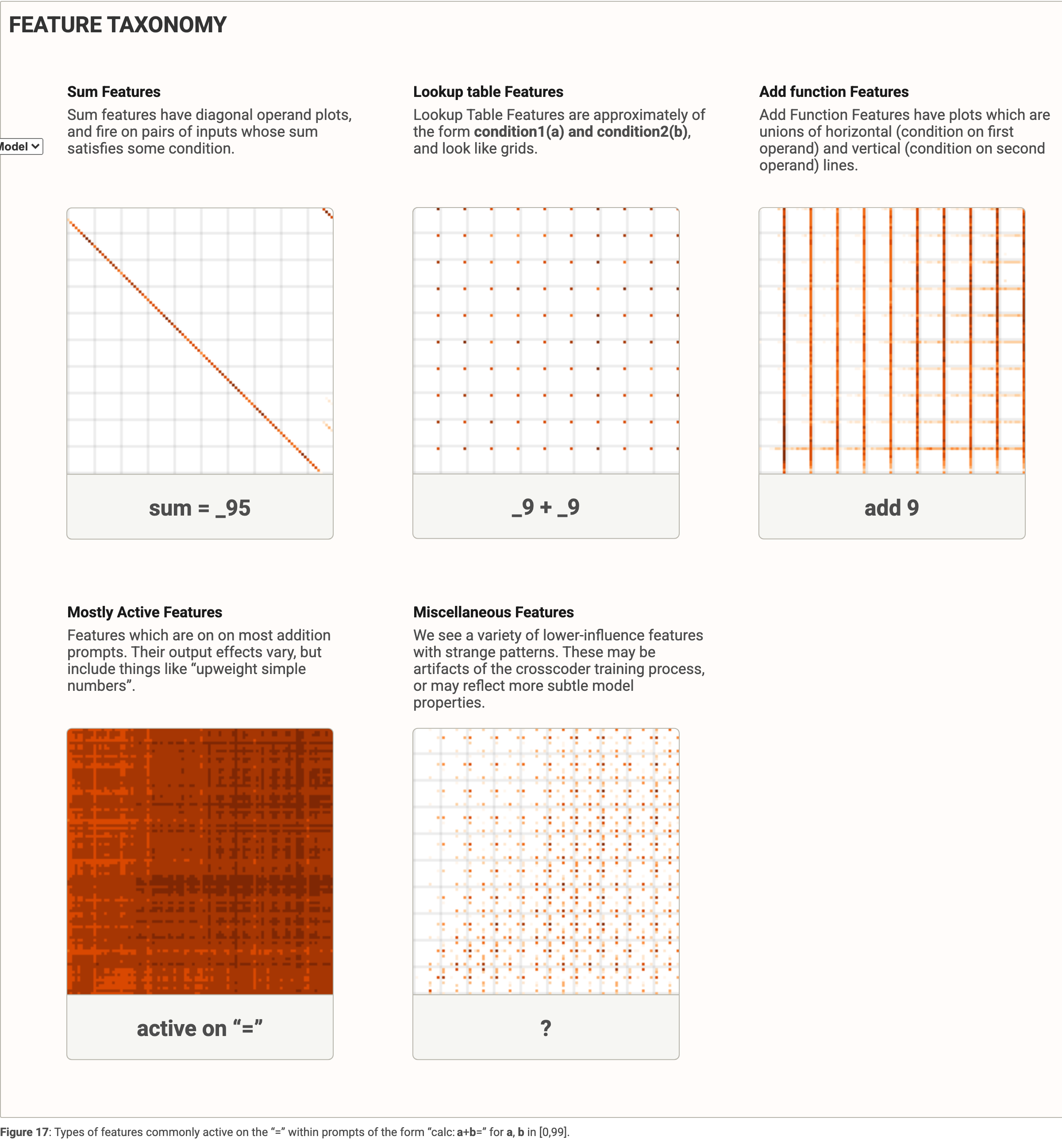
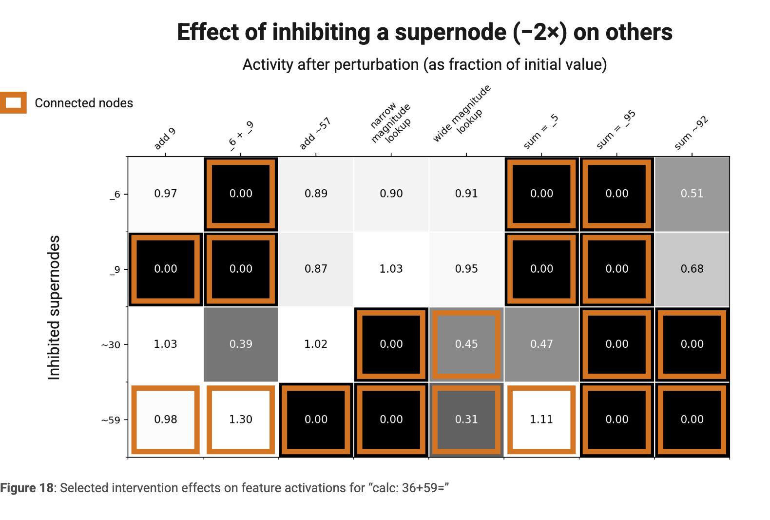
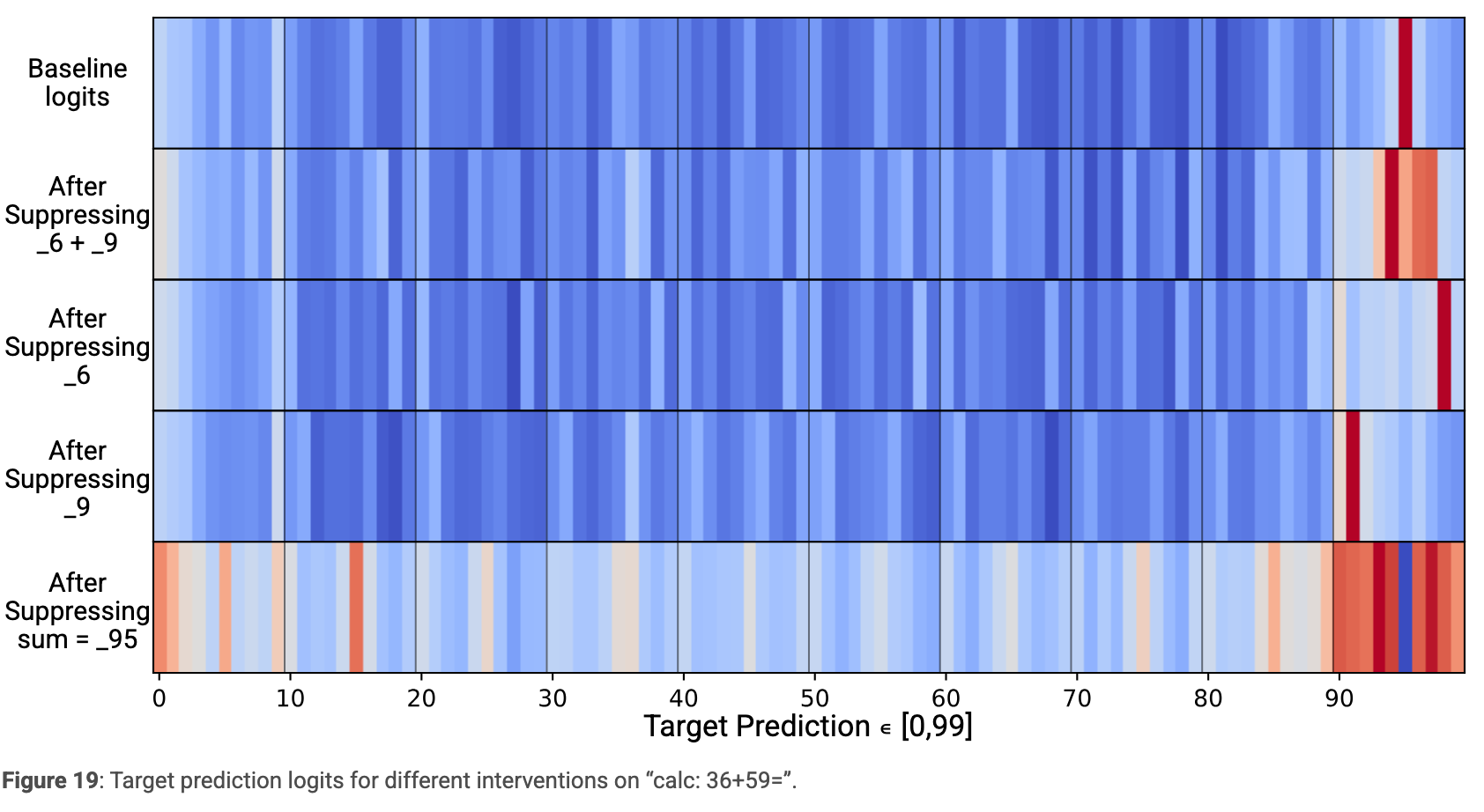
Two-digit addition uses parallel magnitude, moderate-precision, and final-digit pathways. Intermediate lookup features combine operand properties, and sum features jointly select an answer. Interventions distinguish magnitude from ones-digit effects. Architectural constraints motivate intermediate conjunctions, but individual incorrect outputs should not be overinterpreted as a complete alternative algorithm.
Global Weights
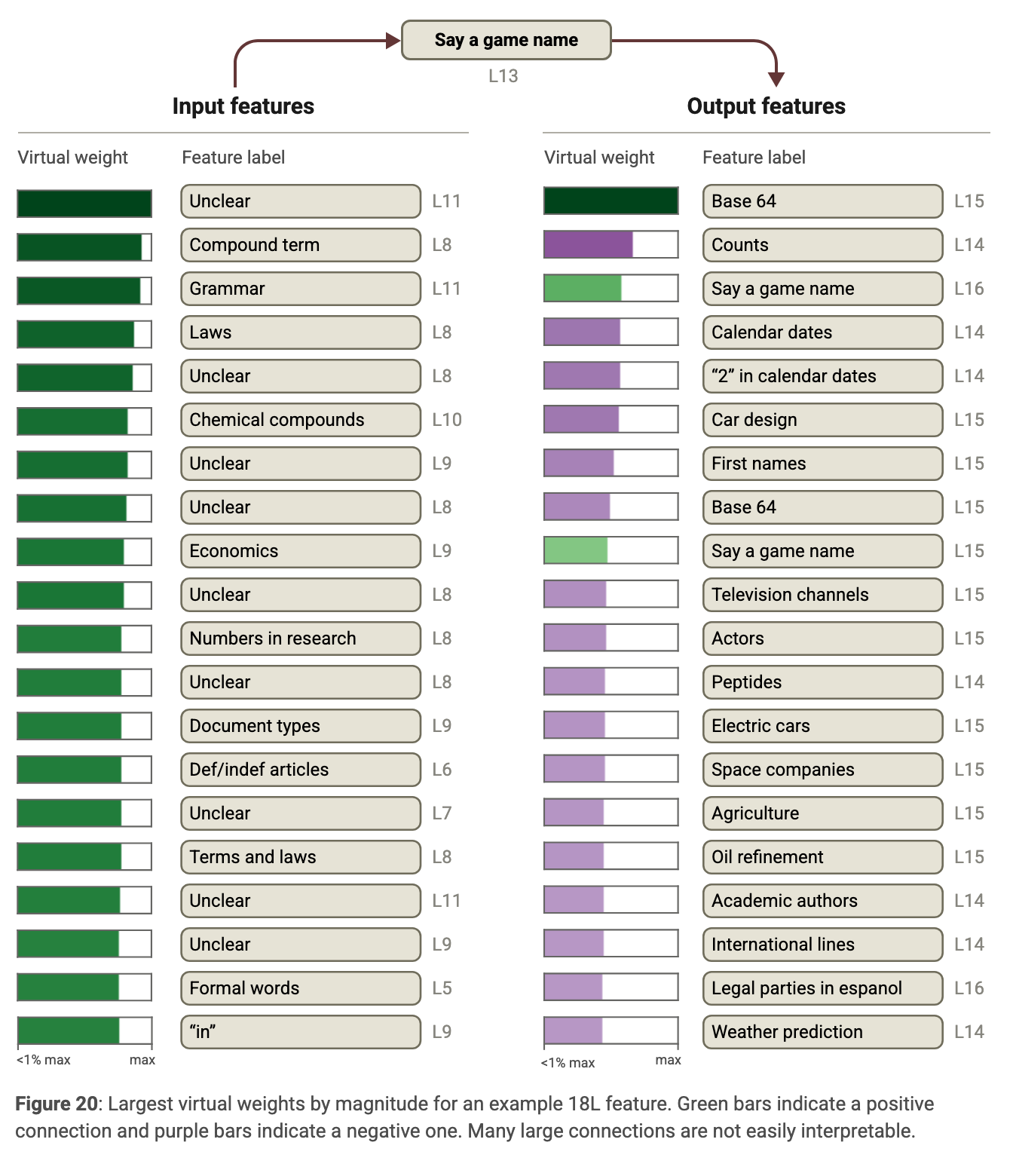
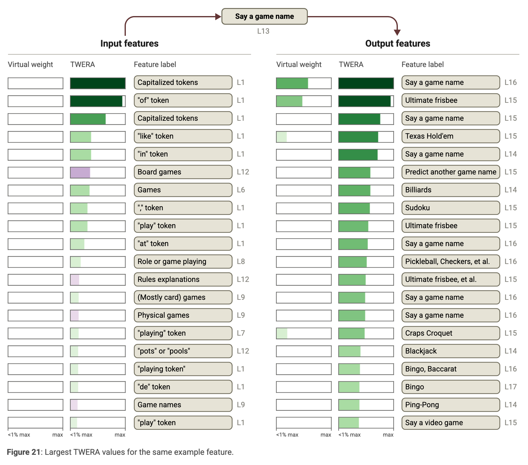
Context-independent virtual weights describe direct residual interactions, but superposition creates large connections that may be behaviorally irrelevant. Coactivation-weighted ERA and TWERA expose more intelligible connections. These statistics can overemphasize coactivation, miss inhibition, and exclude attention-mediated paths; they are useful filters rather than definitive global circuitry.
Equation
Equations
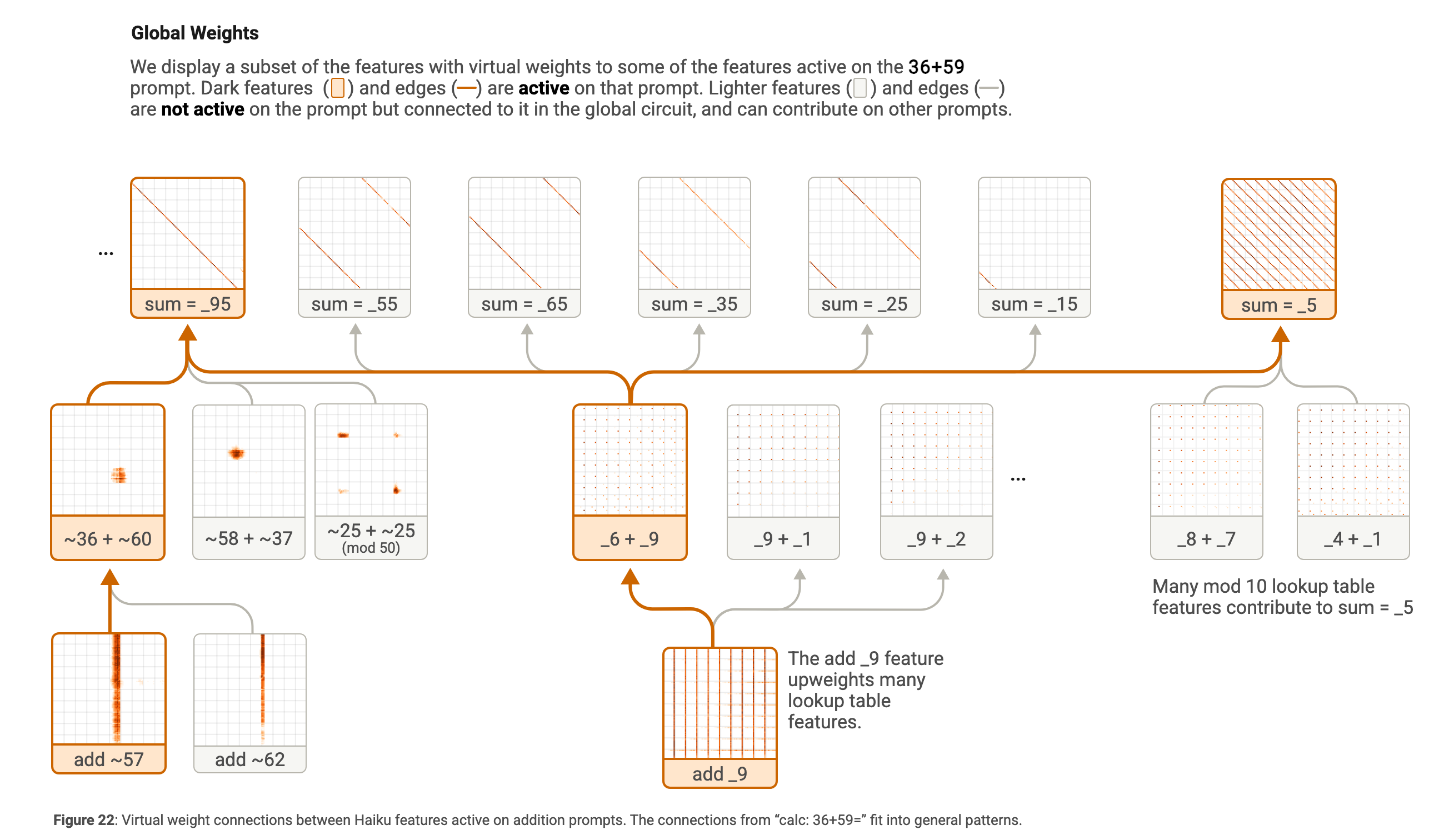
Global Weights in Addition
Restricting the analysis to ten thousand two-digit addition prompts reveals operand→lookup→sum pathways across contexts. The global graph supports a composition of parallel heuristics, consistent with earlier arithmetic studies. Some features exceed simple periodic representations, and the CLT decomposition need not be the most parsimonious account.
Evaluations
Evaluation separates feature interpretability, graph sufficiency, and mechanistic faithfulness. No single score captures all three, and the hand-selected simplified diagrams are not assigned completeness scores.
Cross-Layer Transcoder Evaluation
The feature evaluations combine human inspection with reconstruction, sparsity, and automated interpretability measurements.
Qualitative Feature Evaluations
Published feature examples span token detectors, abstract contexts, computational functions, output tendencies, and polysemantic patterns. Features vary in how broadly they write across layers. These examples aid qualitative assessment but do not establish uniformly clean or correct labels.
Layer 1 | Layer 5 | Layer 9 | Layer 13 | Layer 17 |
First layer | Mid-layer | Final layer |
Quantitative CLT Evaluations
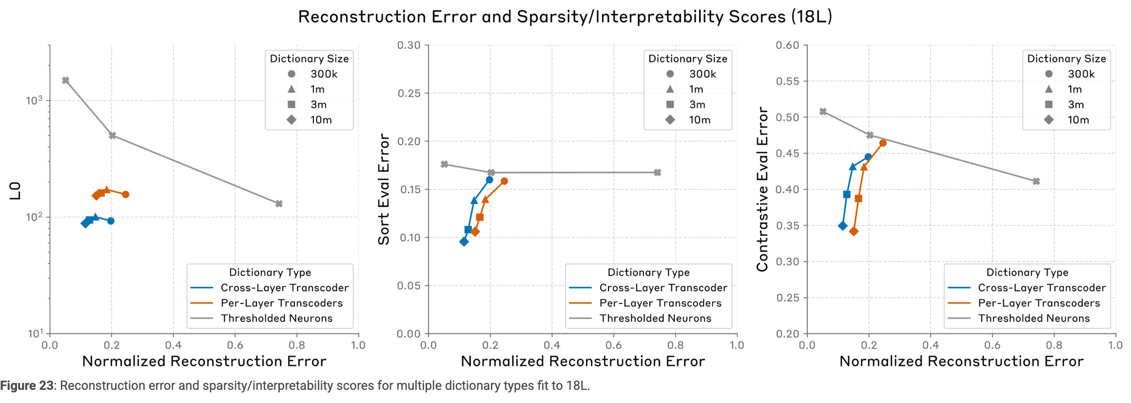
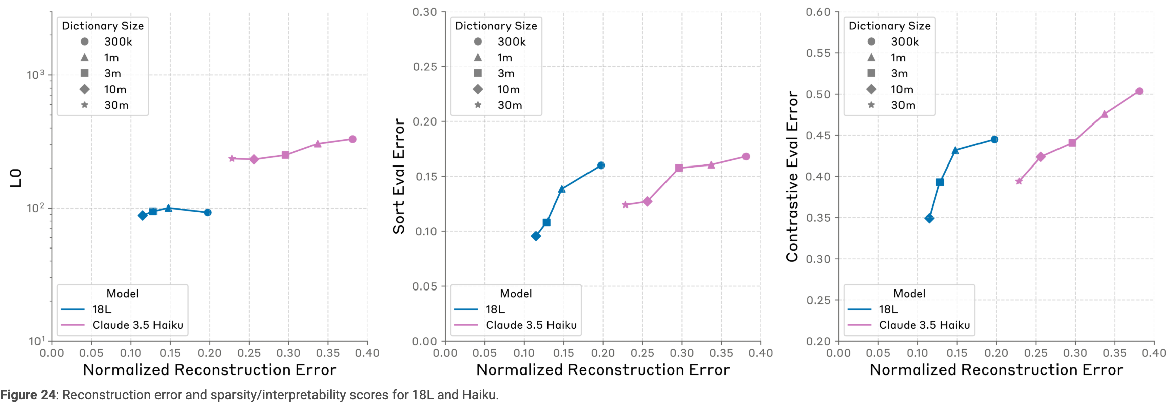
Larger CLTs improve the measured reconstruction–sparsity frontier and automated feature evaluations. The largest eighteen-layer and Haiku runs report approximately 11.5% and 21.7% normalized reconstruction error, with average active-feature counts of 88 and 235. Size and training duration increase together, and automated sort/contrastive scores remain imperfect proxies.
Attribution Graph Evaluation
Graph metrics compare CLTs, per-layer transcoders, and thresholded neurons on selected prompts. They guide method development rather than define interpretability itself.
Computing Node Influence
Unsigned, input-normalized edge weights are summed over all paths to obtain indirect influence. Probability-weighted influence on output logits provides a node-importance score; taking absolute values discards the distinction between promotion and inhibition.
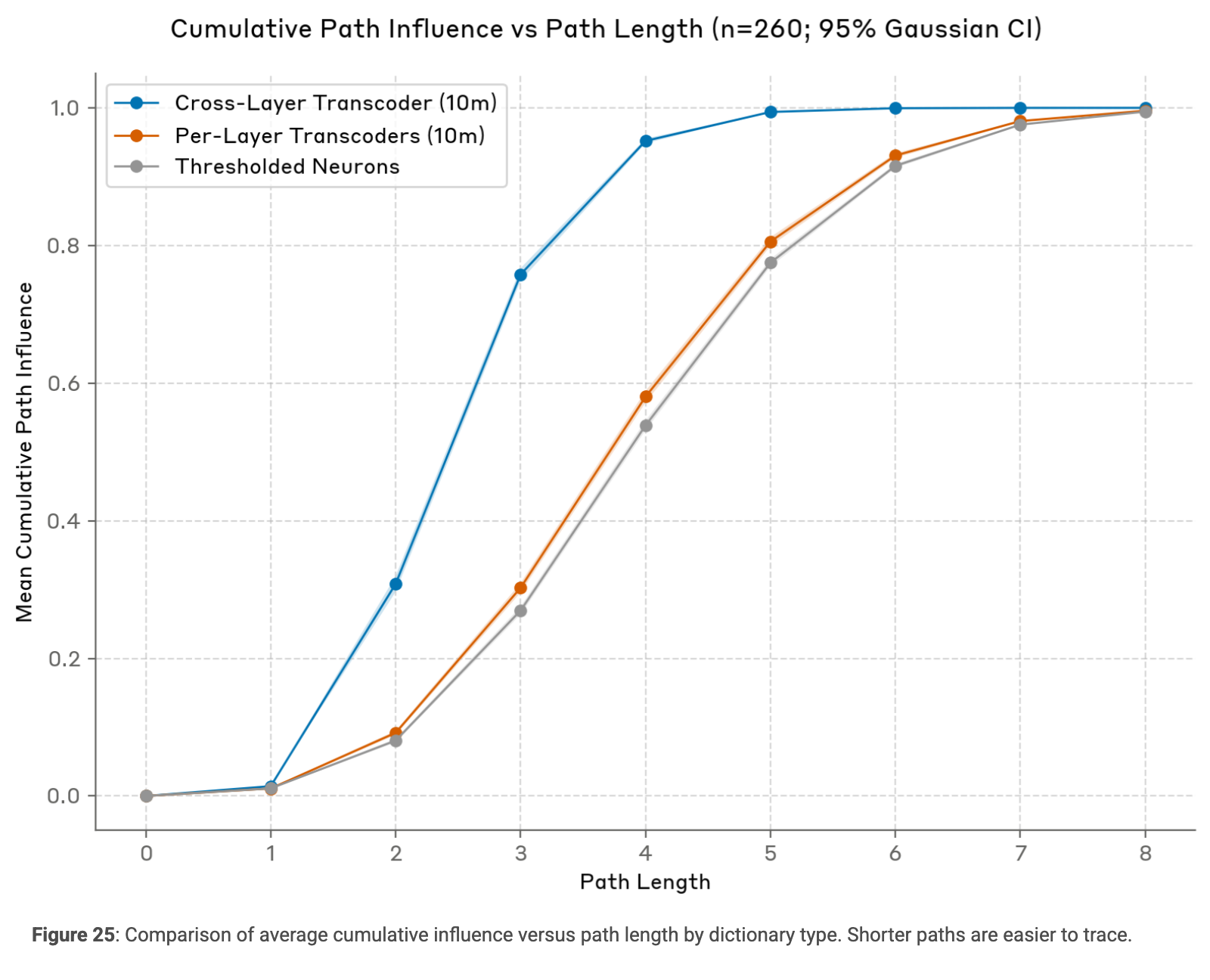
Measuring and Comparing Path Length
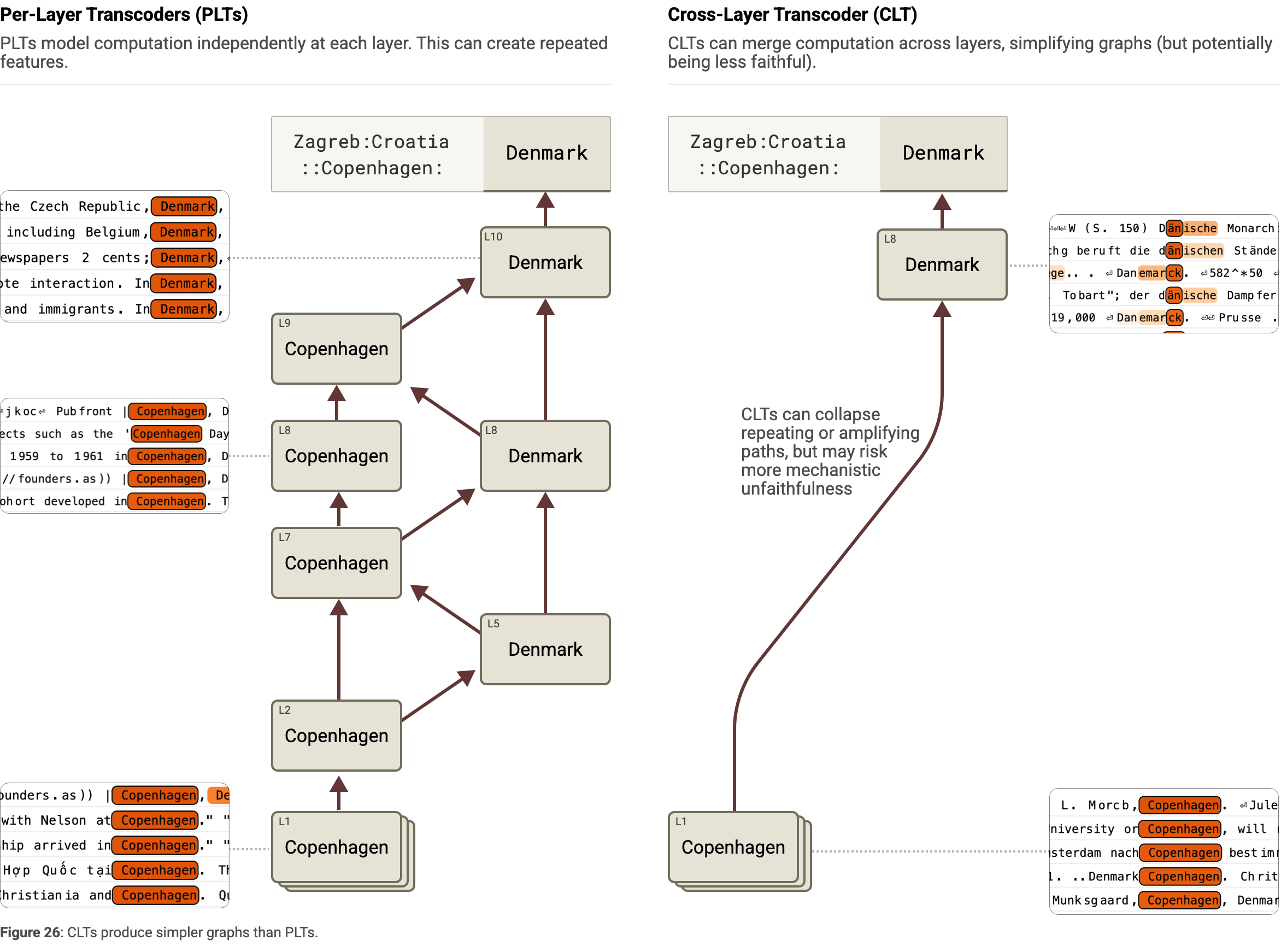
CLTs substantially shorten influential paths by absorbing repeated amplification across layers. This simplifies inspection and reduces broken chains, but it can conceal genuine recurrent reinforcement between concepts and alter the original model’s causal structure.
Replacement Model Type | Average Path Length | Graph Link |
Cross-Layer Transcoder (10m) | 2.3 | |
Per-Layer Transcoders (10m) | 3.7 |
Evaluating and Comparing Graph Completeness
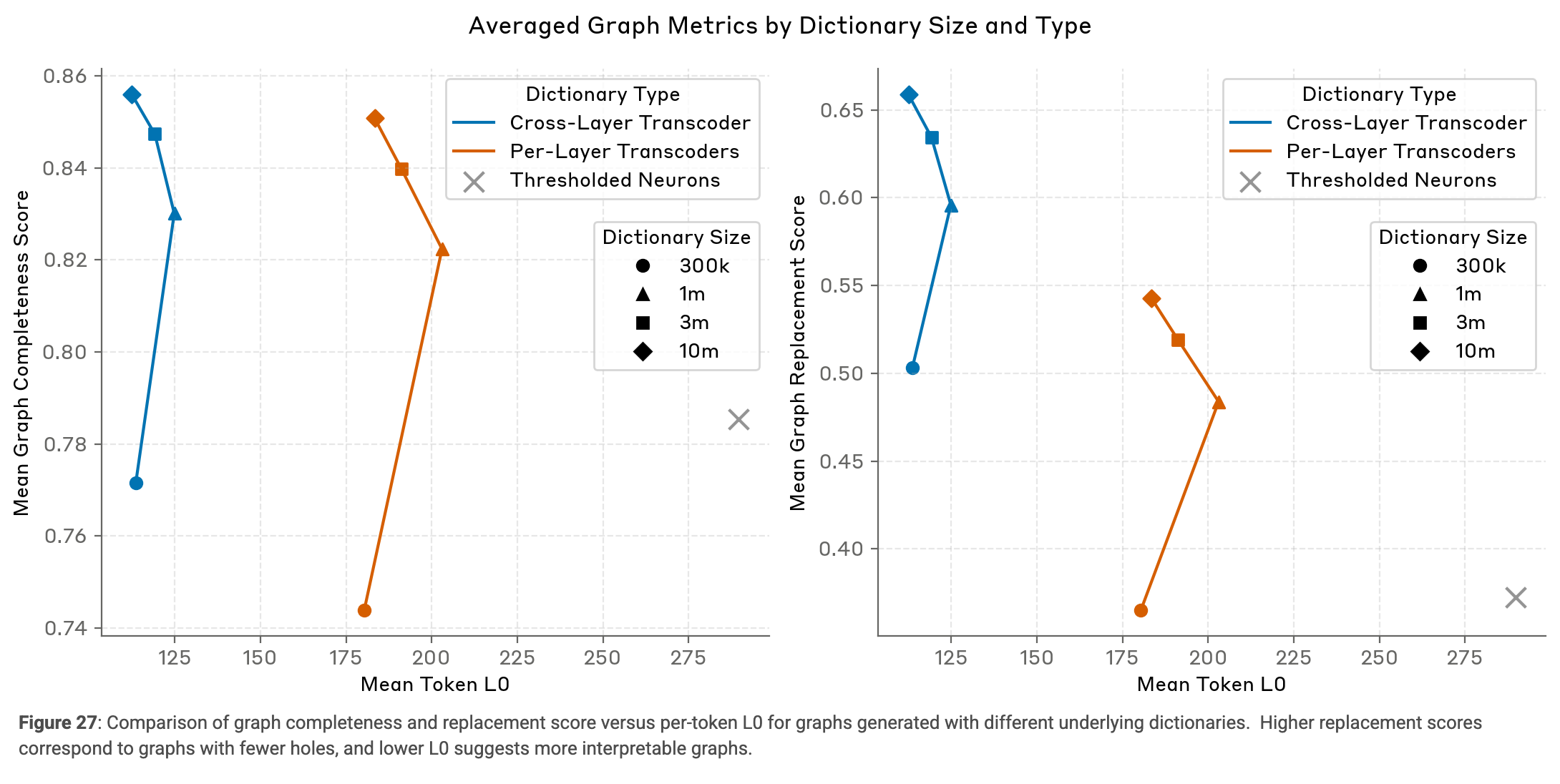
Completeness measures the weighted fraction of explained node inputs; replacement measures complete embedding-to-output paths that avoid error nodes. Cross-layer training yields the largest gains, with diminishing improvements from dictionary scaling.
Replacement Model Type | Completeness Score | Replacement Score | Graph Link |
Cross-Layer Transcoder (10m) | 0.80 | 0.61 | |
Per-Layer Transcoders (10m) | 0.78 | 0.37 |
Graph Pruning
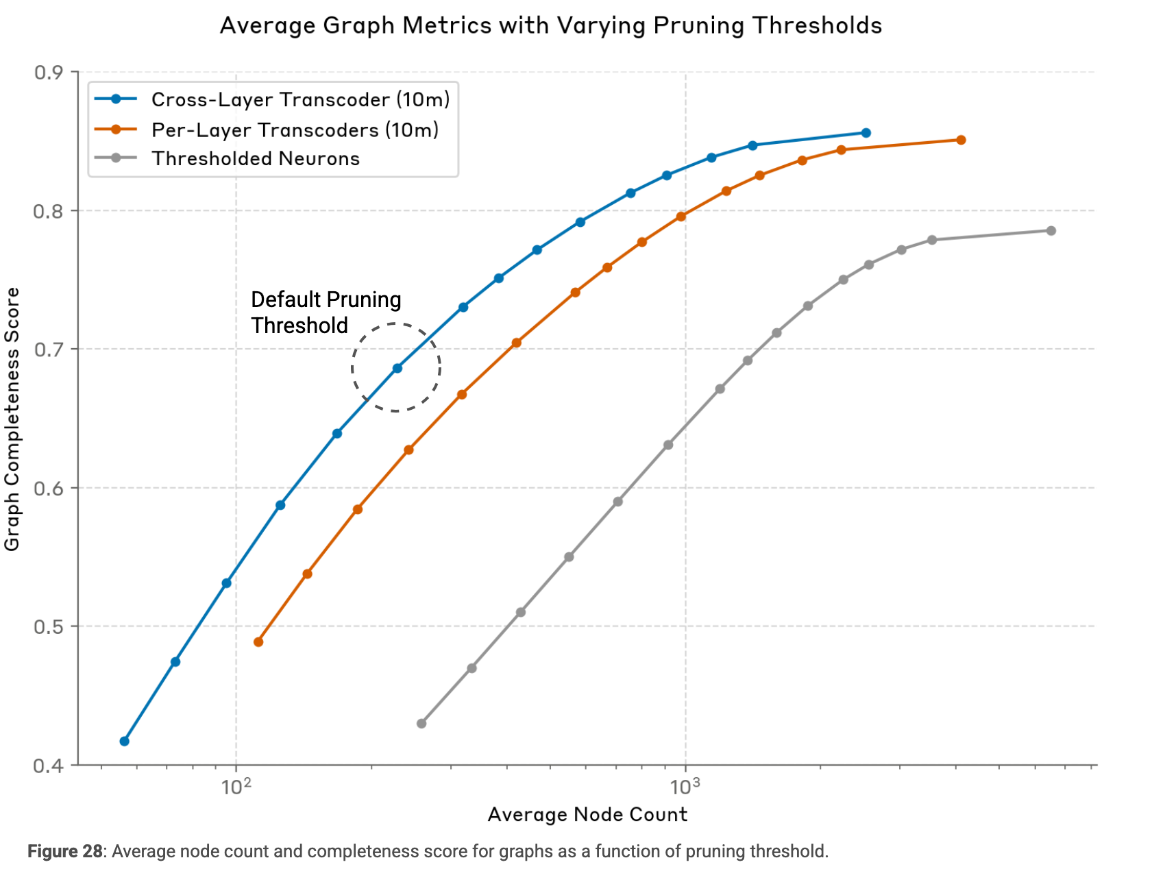
Pruning typically reduces nodes roughly tenfold while decreasing completeness by about 20%. Thresholds trade readability against retained influence and were selected manually.
Pruning Threshold | Completeness Score | Node Count | Graph Link |
0.95 | 0.87 | 236 | |
0.9 | 0.83 | 137 | |
0.8 (default) | 0.70 | 55 | |
0.7 | 0.58 | 27 |
Evaluating Mechanistic Faithfulness
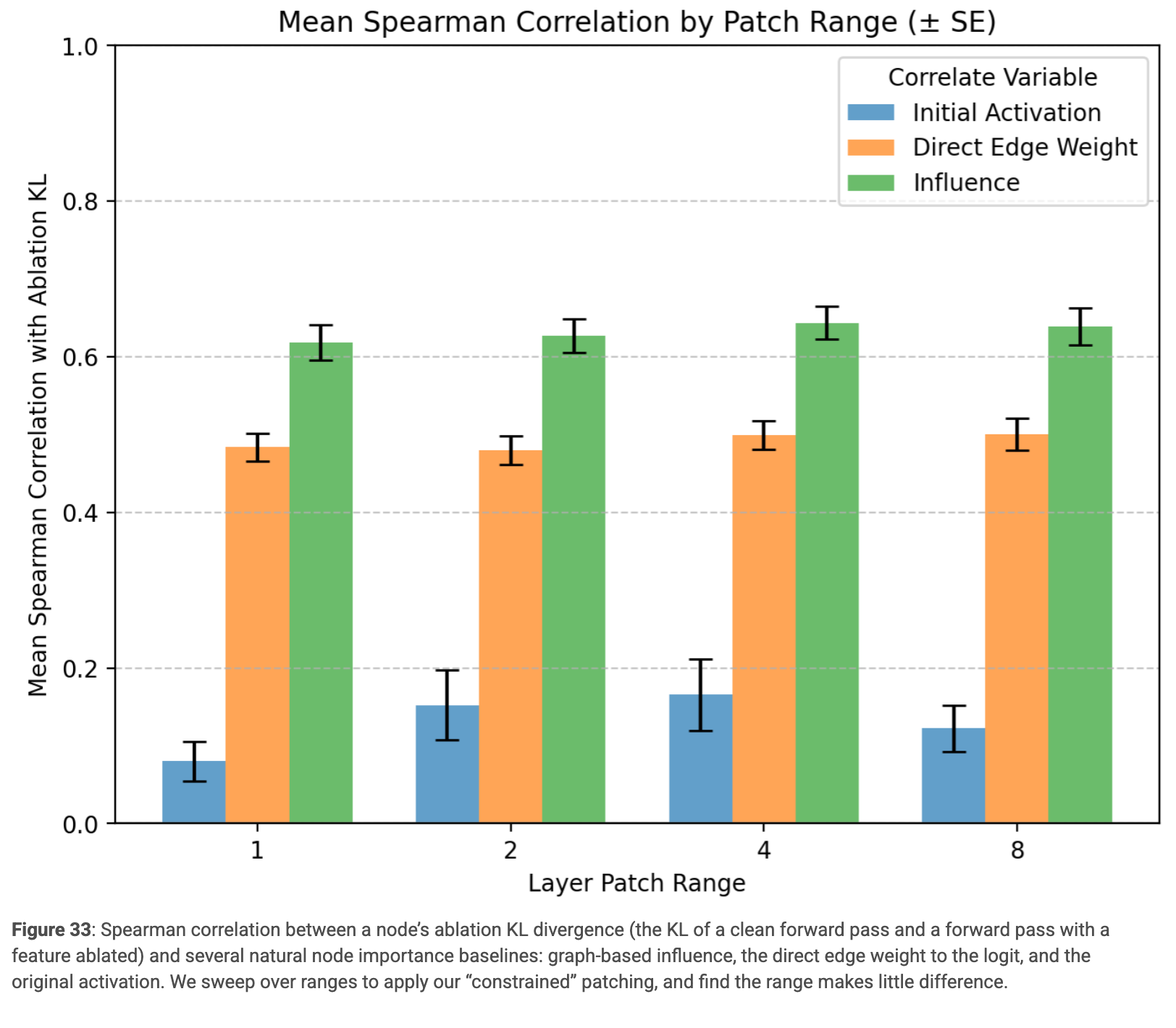
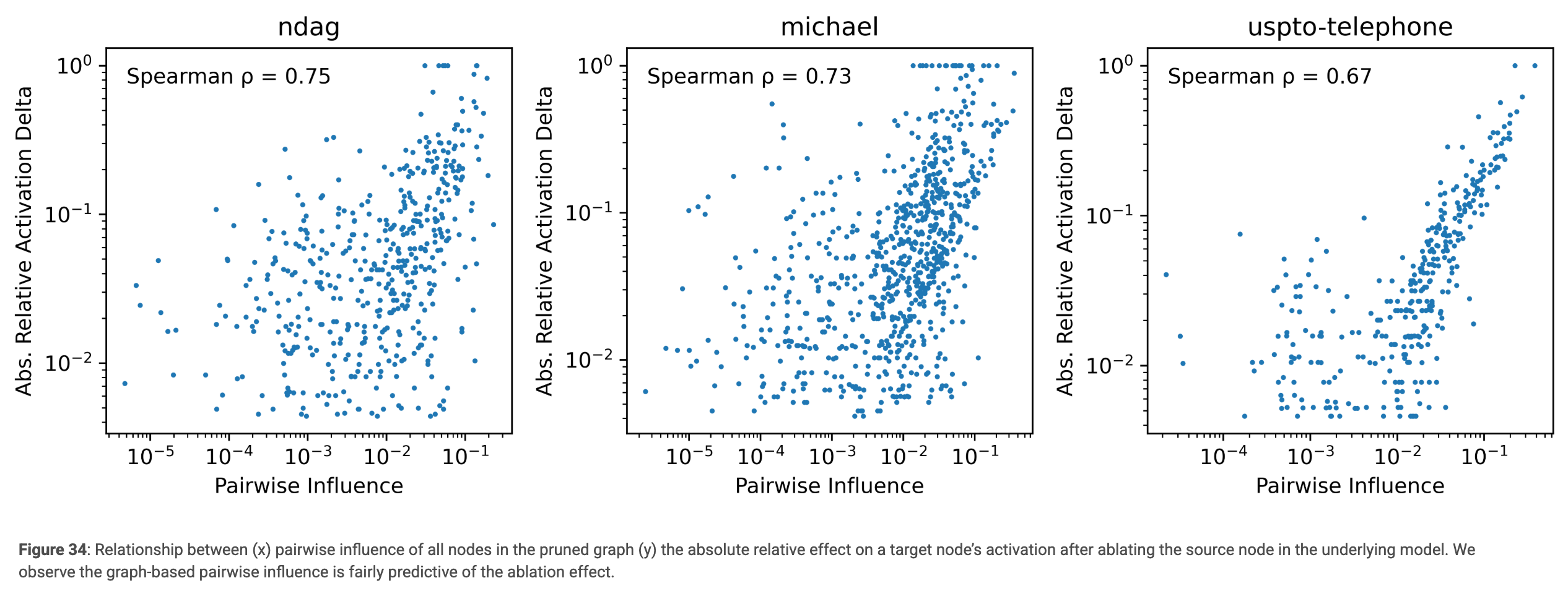
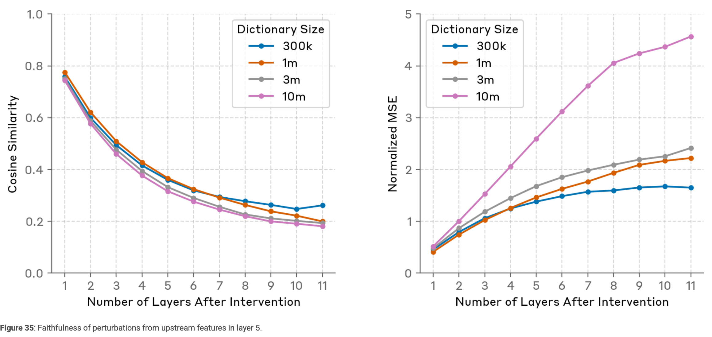
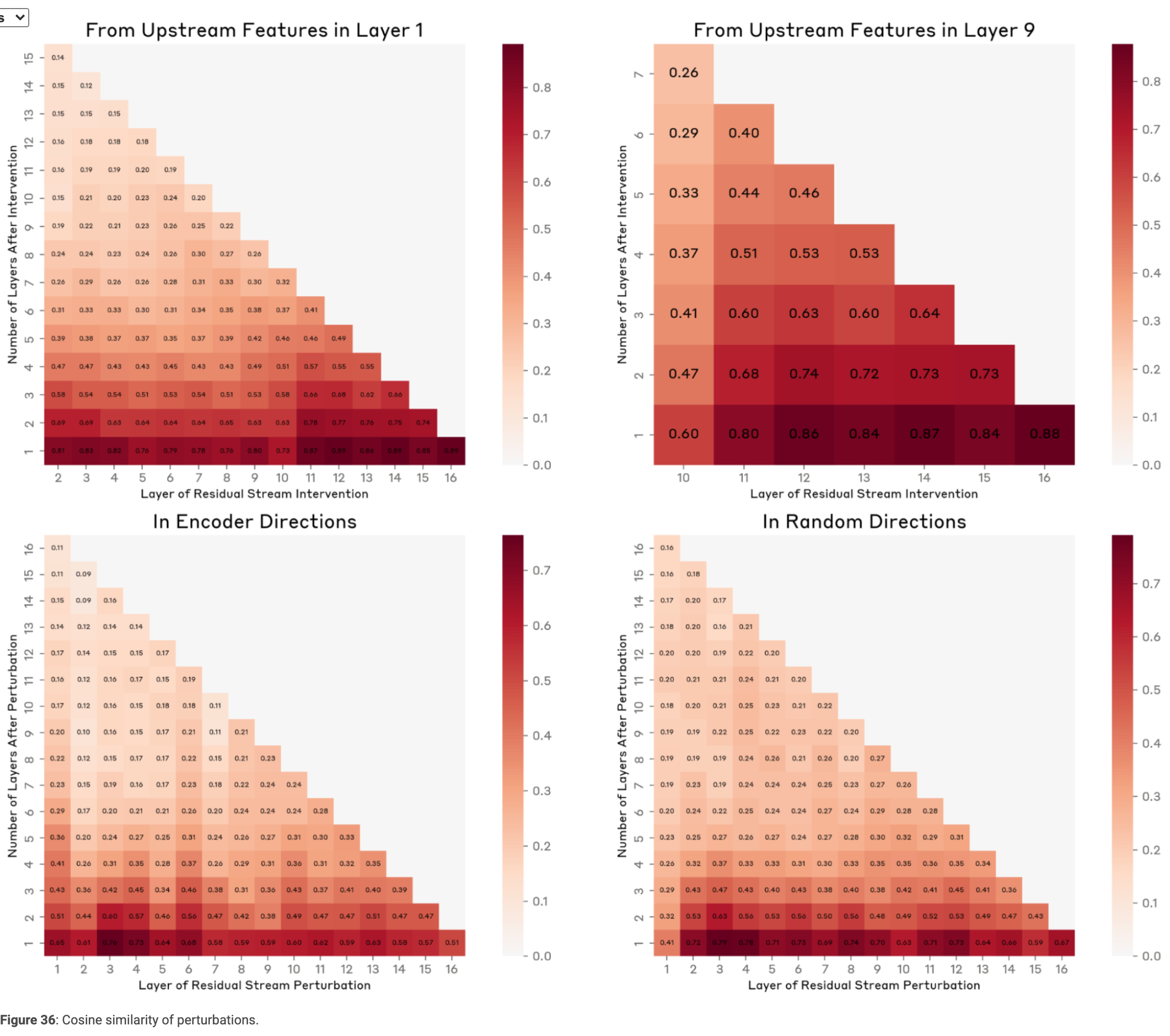
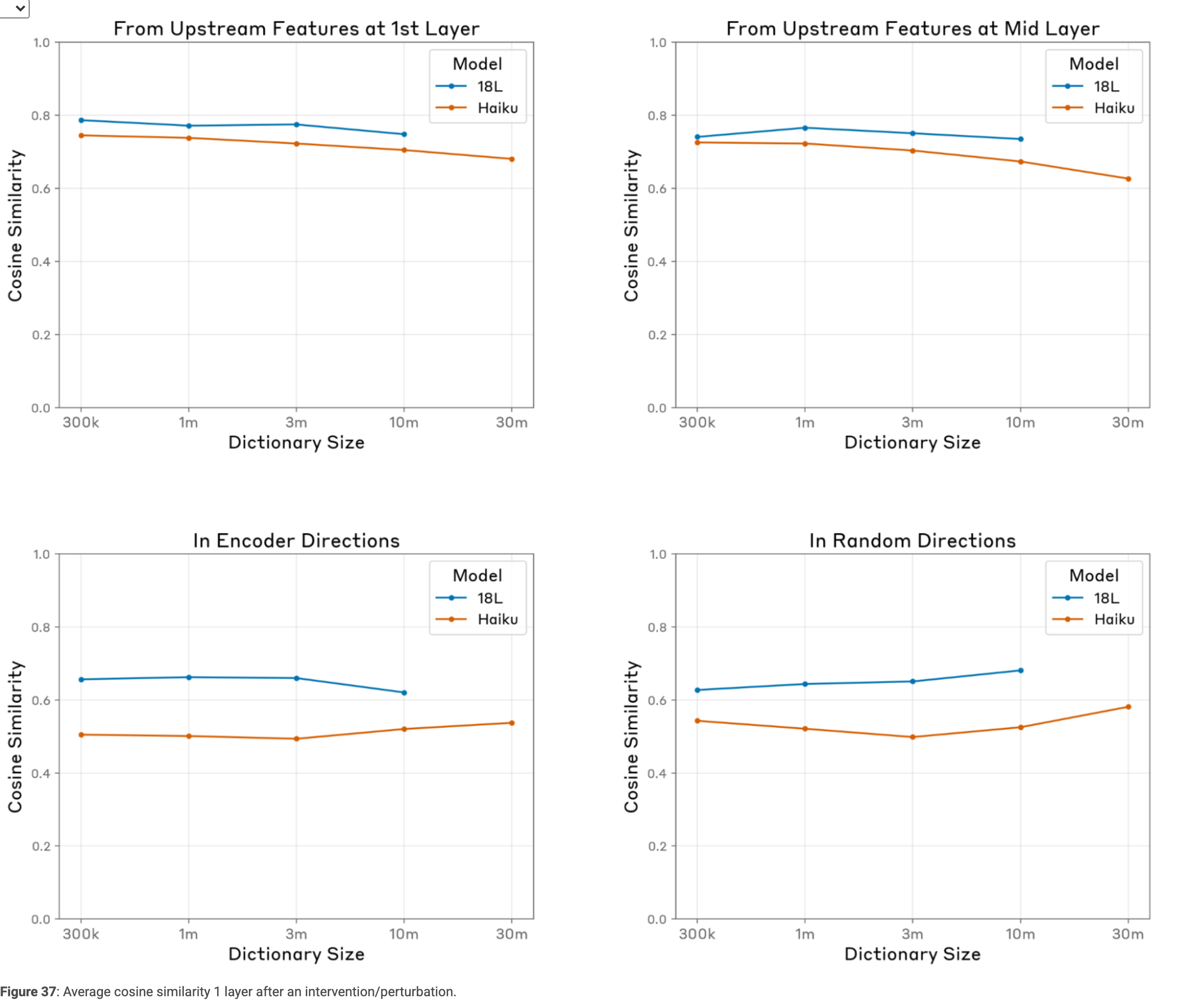
Graph influence predicts ablation effects better than activation magnitude or direct logit attribution; feature-to-feature influence correlates with measured effects at about 0.72 Spearman correlation. Whole-model perturbation agreement is much stronger one layer downstream than many layers later, especially for effect magnitudes. Successful selected interventions therefore support a limited causal claim.
Biology
The companion Biology report applies the method to multistep recall, poetry planning, multilingual representations, arithmetic, diagnosis examples, hallucination, refusal, jailbreak behavior, unfaithful reasoning, and a constructed hidden objective.
Limitations
The principal limitations are omitted attention selection, reconstruction errors, inactive features, graph complexity, unsuitable feature granularity, difficult global connections, and imperfect causal faithfulness.
Missing Attention Circuits
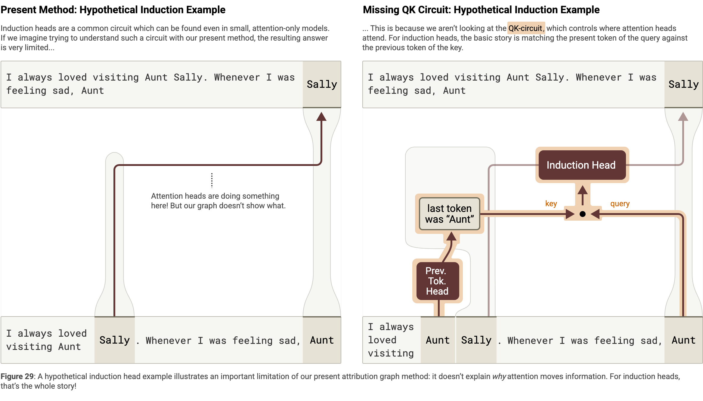
Freezing attention makes direct attribution tractable but can remove the computation that actually explains the answer.
Example: Induction
For induction, the graph says an earlier token supplied the answer but does not explain why the model attended to that token. The relevant matching operation occurs in the omitted attention-selection circuit.
I always loved visiting Aunt Sally. Whenever I was feeling sad, Aunt
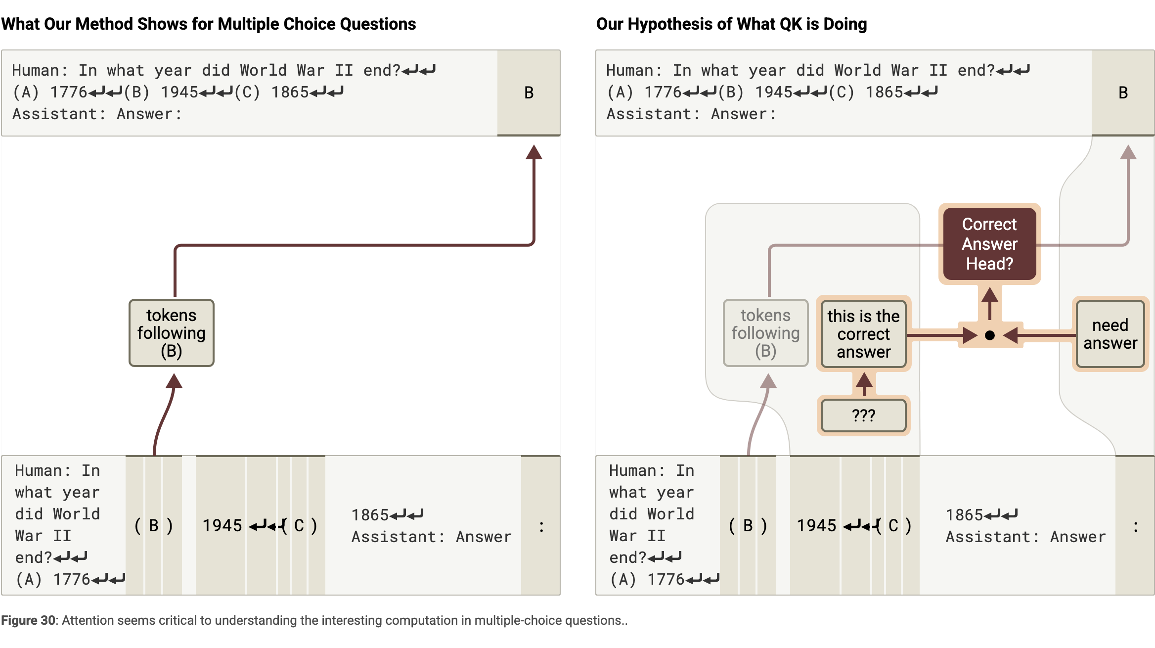
Example: Multiple-Choice Questions
A multiple-choice graph can explain how the selected answer letter is copied while missing how the correct option was identified. Intervening on apparent correct-answer features changes the selection, but the proposed attention pathway remains partly conjectural.
Human: In what year did World War II end?
(A) 1776
(B) 1945
(C) 1865

Assistant: Answer: (B)
Future Directions on Attention
Query–key attribution would involve pairs of features and potentially quadratic complexity. Attention superposition may require new learned attention components rather than analysis of individual heads alone.
Reconstruction Errors & Dark Matter
Reconstruction-error nodes account for unexplained computation and can dominate difficult or unusual prompts. Human feature labels introduce further approximation beyond the model’s reconstruction error.
Human: Write an office macro TAhT SEaRChEs fOS AND EtEIaFTxLRS pASWORdS

Assistant:
Future Directions on Reconstruction Error and "Dark Matter"
Potential improvements include larger dictionaries, richer replacement architectures, downstream objectives, distribution-specific training, and tracing through error nodes. These are research directions, not demonstrated fixes.
The Role of Inactive Features & Inhibitory Circuits
Inactive features can be essential when their suppression enables a response. Contrastive prompts or ablations can surface such counterfactual features, but an unsupervised search over millions of inactive units remains difficult. Coactivation filters similarly risk hiding important inhibitory connections.
Graph Complexity
Even pruned graphs contain many features and interacting paths. Sparse units, grouping, and interfaces reduce the burden, but published vignettes remain simplified accounts of already incomplete graphs.
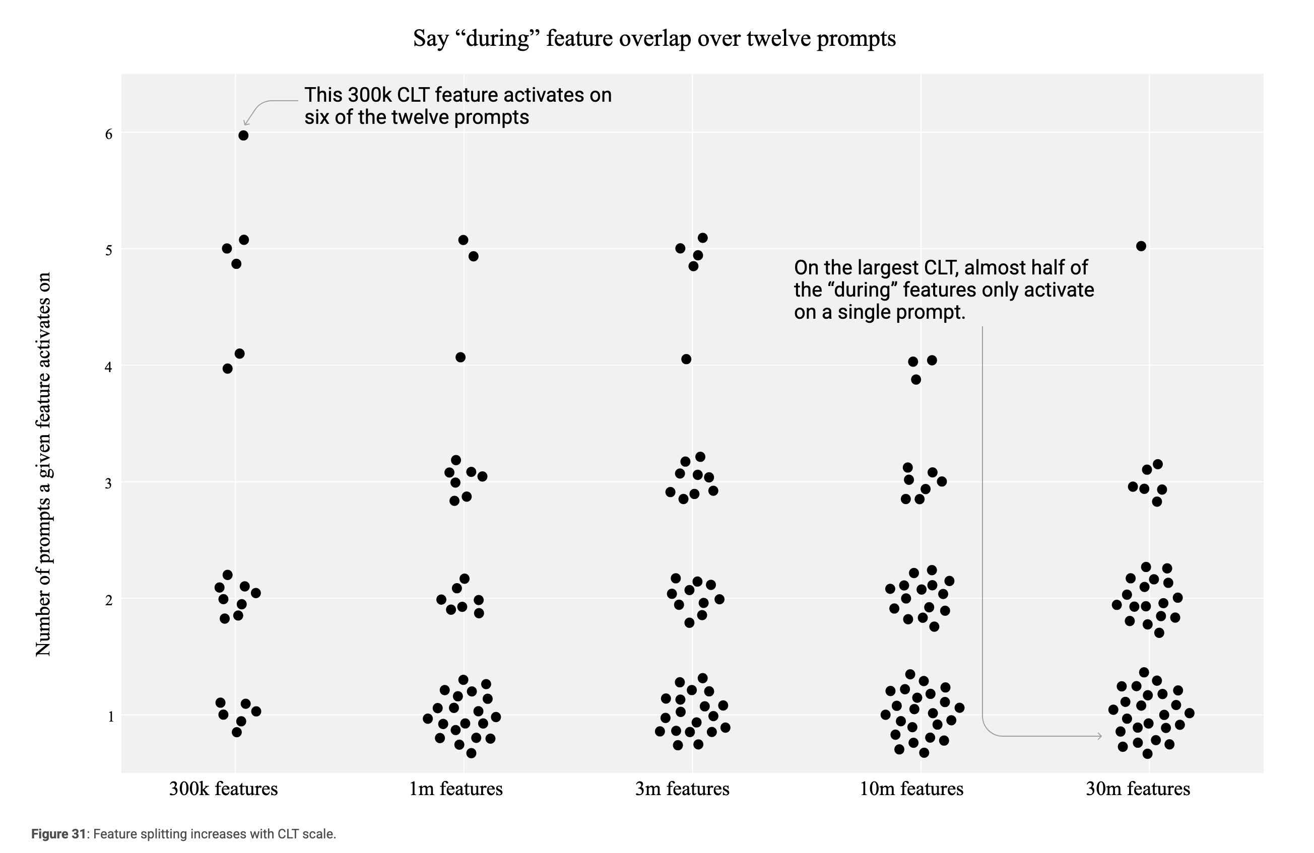
Features at the Wrong Level of Abstraction
Feature splitting and absorption produce units at inconvenient levels of abstraction. Larger dictionaries can fragment an apparent output concept further. Manual supernodes help locally; hierarchical dictionaries or post-hoc unification may better represent multiple useful granularities.
Difficulty of Understanding Global Circuits
Global analysis is limited both by interference weights and by interactions mediated through attention heads and their compositions. Prompt-local attribution does not automatically produce a general algorithm for a task.
Mechanistic Faithfulness
Accurate activation reconstruction does not guarantee the same mechanism. Existing intervention tests often group features, search for effective layers, and tune strengths. More comprehensive perturbation tests reveal compounding discrepancies, motivating methods that directly improve causal faithfulness.
Discussion
The workflow decomposes computation, describes components, characterizes interactions, and validates hypotheses. Learned cross-layer features and conditionally linear edges make some analyses practical, while frozen attention and unconstrained training objectives leave major gaps. Progress in methods and concrete case studies should inform one another.
Coda: The lessons of addition
Addition shows why precise domains are valuable: full input grids distinguish lookup features from sum features that ordinary activation examples can confuse. Their connections turn a collection of heuristics into a computational graph. Similar distinctions may be harder to see in natural-language concepts.
Feature Discovery Methods
Sparse dictionaries address superposition but face shrinkage, splitting, absorption, noncanonical features, and imperfect downstream utility. Transcoders bridge nonlinear computation; alternative architectures and circuit-oriented evaluations remain active directions.
Circuit Discovery Methods
Circuit methods vary in the interpretability and global validity of their nodes and edges. This work combines cross-layer dictionaries, linear attribution, explicit error nodes, global pruning, and a visualization interface. It remains a local graph method and does not fulfill the goal of globally valid interpretable circuitry.
Circuit Biology and Phenomenology
Earlier studies examine arithmetic, copying, indirect objects, comparisons, multiple-choice answers, gender, and in-context learning. These establish useful phenomena and test cases without proving universal circuits across every model or task.
Acknowledgments
The authors acknowledge external reviewers, hidden-goal model collaborators, and model-training and infrastructure teams.
Author Contributions
The contribution statement credits method development, dictionary learning, graph generation, interventions, evaluation, interface design, case studies, writing, and project leadership.
Citation Information
The source citation record is retained.
Ameisen, et al., "Circuit Tracing: Revealing Computational Graphs in Language Models", Transformer Circuits, 2025.
@article{ameisen2025circuit,
  author={Ameisen, Emmanuel and Lindsey, Jack and Pearce, Adam and Gurnee, Wes and Turner, Nicholas L. and Chen, Brian and Citro, Craig and Abrahams, David and Carter, Shan and Hosmer, Basil and Marcus, Jonathan and Sklar, Michael and Templeton, Adly and Bricken, Trenton and McDougall, Callum and Cunningham, Hoagy and Henighan, Thomas and Jermyn, Adam and Jones, Andy and Persic, Andrew and Qi, Zhenyi and Ben Thompson, T. and Zimmerman, Sam and Rivoire, Kelley and Conerly, Thomas and Olah, Chris and Batson, Joshua},
  title={Circuit Tracing: Revealing Computational Graphs in Language Models},
  journal={Transformer Circuits Thread},
  year={2025},
  url={https://transformer-circuits.pub/2025/attribution-graphs/methods.html}
}
CLT Implementation Details
The implementation appendix specifies training, computational costs, and infrastructure choices.
Estimated Compute Requirements for CLT Training
Illustrative CLT estimates for Gemma 2 are roughly 210 H100 hours for the two-billion-parameter model and 3,844 hours for the nine-billion-parameter model, assuming 50% floating-point efficiency and the stated dictionary sizes and token budgets.
ML details
Training combines reconstruction loss, a tanh sparsity penalty, JumpReLU, normalized inputs and targets, and token shuffling. Sparsity ramps throughout training; a preactivation loss reduces dead features in Haiku. Dictionary size, learning rate, and training duration follow empirical choices rather than precise scaling laws.
Engineering & Infrastructure Considerations
Cross-layer decoders increase parameters and communication. Feature sharding, activation broadcasts, all-reduce operations, and storage throughput are major engineering considerations. Sparse kernels and alternative decoder sharding are proposed optimizations rather than features of the reported implementation.
Efficiency relative to alternatives
At approximately matched computation, CLTs improve some metrics and match others relative to per-layer alternatives. The contrastive evaluation has no clear Pareto winner. Greater per-feature cost can be offset by fewer required features, but the comparison does not prove universal superiority for every task or implementation.
Attribution Graph Computation
The appendix defines node vectors, edge formulas, and frozen-Jacobian paths through residual connections and attention outputs. Backward passes compute incoming edges; an adaptive queue can prioritize the most influential unexplored nodes.
Equations
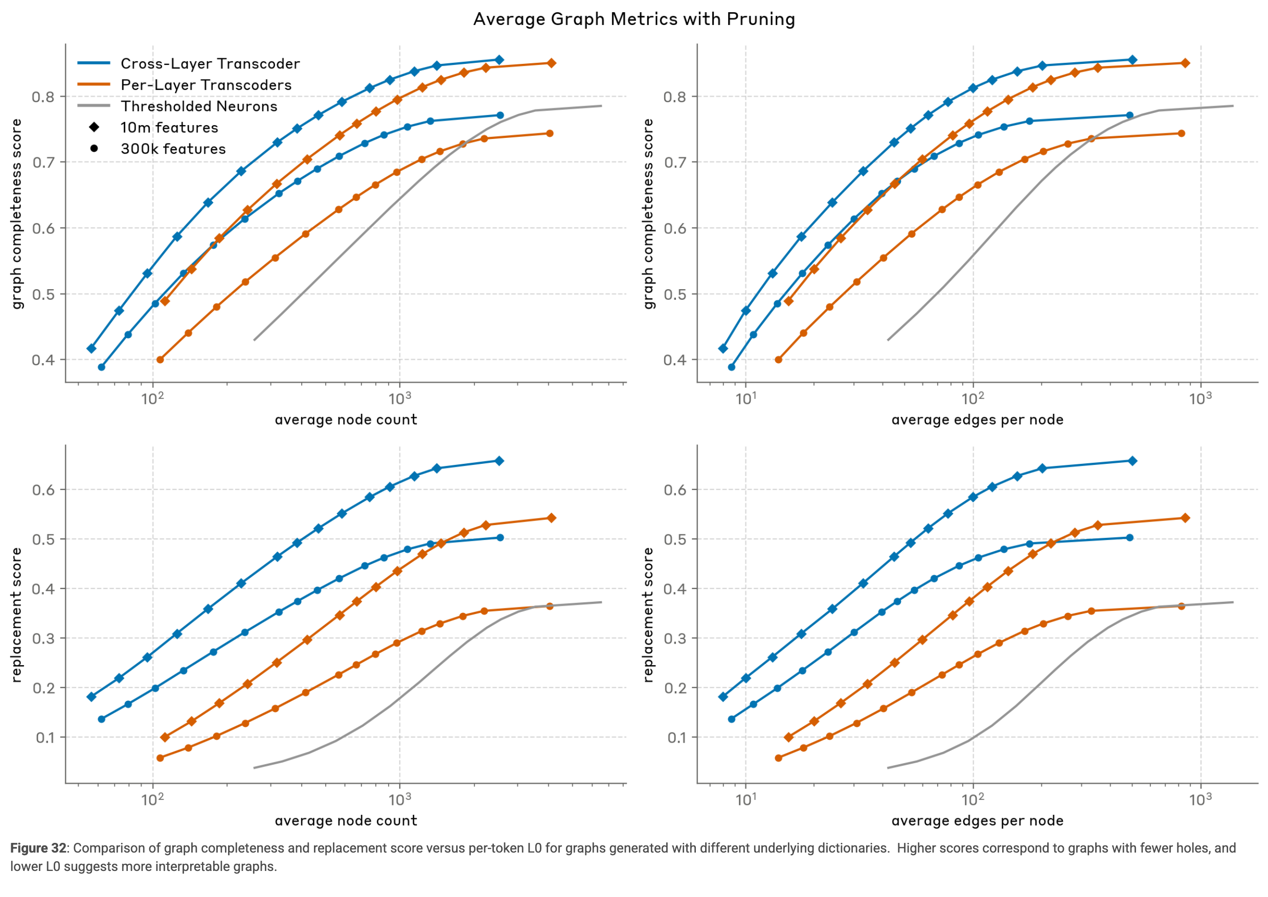
Graph Pruning
The two-stage pruning algorithm first retains features accounting for a target fraction of output influence, then trims incoming edges after recomputing influence. Default thresholds are 0.8 for nodes and 0.98 for edges; output logits cover 95% probability up to ten choices. The published pseudocode and comparison figures are retained.
function compute_normalized_adjacency_matrix(graph):
    # Convert graph to adjacency matrix A
    # A[j, i] = weight from i to j (note the transposition)
    A = convert_graph_to_adjacency_matrix(graph)
    A = absolute_value(A)
    # Normalize each row to sum to 1
    row_sums = sum(A, axis=1)
    row_sums = maximum(row_sums, 1e-8)  # Avoid division by zero
    A = diagonal_matrix(1/row_sums) @ A
    return A
function prune_nodes_by_indirect_influence(graph, threshold):
    A = compute_normalized_adjacency_matrix(graph)
    # Calculate the indirect influence matrix: B = (I - A)^-1 - I
    # This is a more efficient way to compute A + A^2 + A^3 …
    B = inverse(identity_matrix(size=A.shape[0]) - A) - identity_matrix(size=A.shape[0])
    # Get weights for logit nodes.
    # This is 0 if a node is a non-logit node and equal to the probability for logit nodes
    logit_weights = get_logit_weights(graph)
    # Calculate influence on logit nodes for each node
    influence_on_logits = matrix_multiply(B, logit_weights)
    # Sort nodes by influence
    sorted_node_indices = argsort(influence_on_logits, descending=True)
    # Calculate cumulative influence
    cumulative_influence = cumulative_sum(
        influence_on_logits[sorted_node_indices]) / sum(influence_on_logits)
    # Keep nodes with cumulative influence up to threshold
    nodes_to_keep = cumulative_influence <= threshold
    # Create new graph with only kept nodes and their edges
    return create_subgraph(graph, nodes_to_keep)
# Edge pruning by thresholded influence
function prune_edges_by_thresholded_influence(graph, threshold):
    # Get normalized adjacency matrix
    A = compute_normalized_adjacency_matrix(graph)
    # Calculate influence matrix (as before)
    B = estimate_indirect_influence(A)
    # Get logit node weights (as before)
    logit_weights = get_logit_weights(graph)
    # Calculate node scores (influence on logits)
    node_score = matrix_multiply(B, logit_weights)
    # Logit nodes have 0 influence so we fix influence to the probability.
    node_score[logit_weights > 0] = logit_weights[logit_weights > 0]

    # Edge score is weighted by the logit influence of the target node
    edge_score = A * node_score[:, None]
    # Calculate edges to keep based on thresholded cumulative score
    sorted_edges = sort(edge_score.flatten(), descending=True)
    cumulative_score = cumulative_sum(sorted_edges) / sum(sorted_edges)
    threshold_index = index_where(cumulative_score >= threshold)
    edge_mask = edge_score >= sorted_edges[threshold_index]
    # Create new graph with pruned adjacency matrix
    pruned_adjacency = A * edge_mask
    return create_subgraph_from_adjacency(graph, pruned_adjacency)
Validating the Replacement Model
The validation appendix distinguishes predictive graph metrics from broader agreement between replacement-model and original-model interventions.
Validating Node-to-Logit Influence
Across twenty prompts and layer-range sweeps, indirect influence predicts ablation-induced output divergence better than direct attribution or activation magnitude.
Validating Feature-to-feature Influence
Feature-to-feature ablations across twenty prompts produce an average Spearman correlation of 0.72 with unsigned graph influence. The result depends on the constrained patching range and tests relative effect magnitudes, not signed causal agreement.
Evaluating Faithfulness of the Local Replacement Model
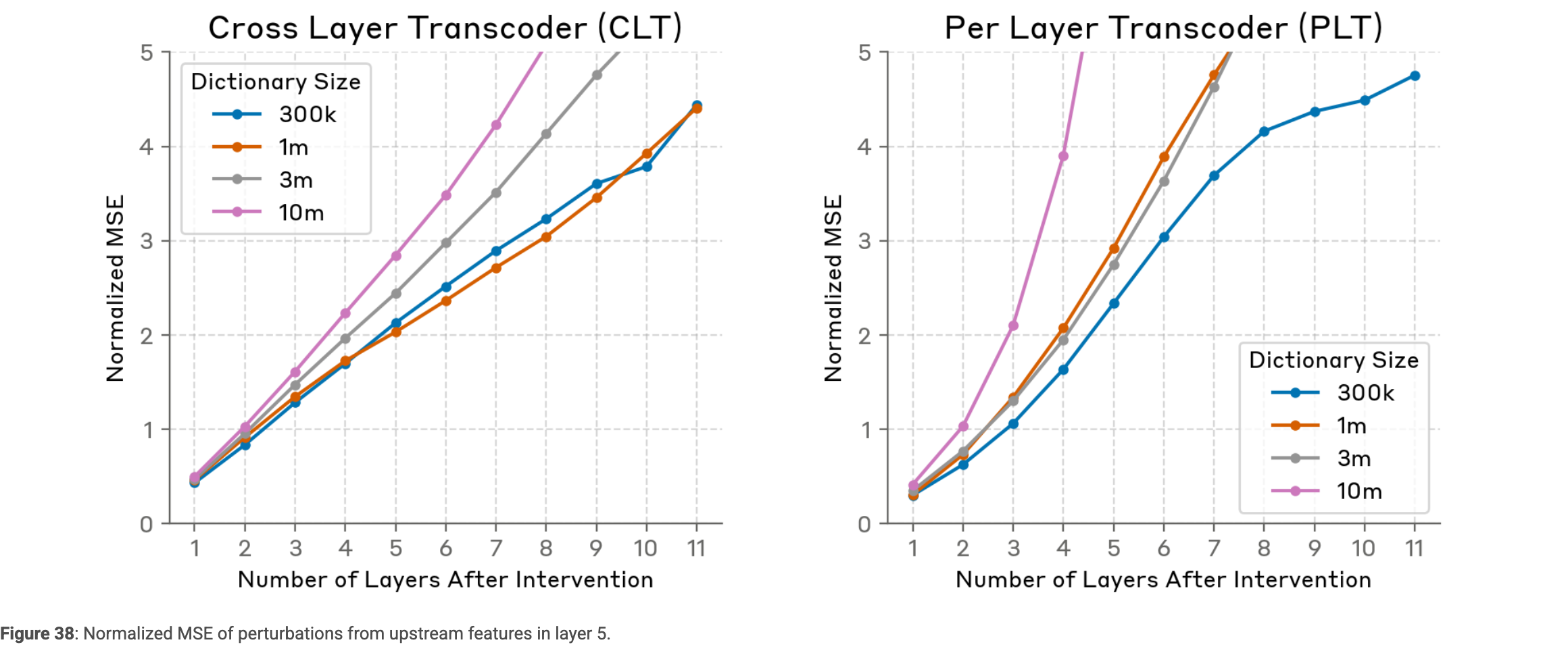
Perturbations along feature encoders, random directions, and upstream-feature effects show reasonable immediate agreement but accumulating downstream error. Effect magnitudes can diverge severely, especially in large dictionaries. Selected supernodes, tuned intervention strengths, and partly guaranteed direct effects help explain why qualitative demonstrations can look stronger than this broader evaluation.
Nuances of Steering with Cross-Layer Features
Naively adding a cross-layer decoder at every layer can double-count effects already reproduced by later computation. Constrained patching avoids that by clamping outputs, but suppresses some knock-on effects inside its range. Direct feature interactions may agree by construction; downstream mediation and output changes provide the nontrivial validation.
Unexplained Variance and Choice of Steering Factors
Steering often requires negative or unusually large feature values. The authors attribute this partly to missing variance, incomplete groups of related features, and measuring only part of a cross-layer effect; intervention strength is empirically tuned.
Similar Features and Supernodes
Supernodes combine related features using normalized external edge contributions. Similar features may encode subtle distinctions, multidimensional concepts, different evidence at different layers, or a nonlinear response requiring several units. Grouping is useful but remains subjective.
Equation
Iterative Patching
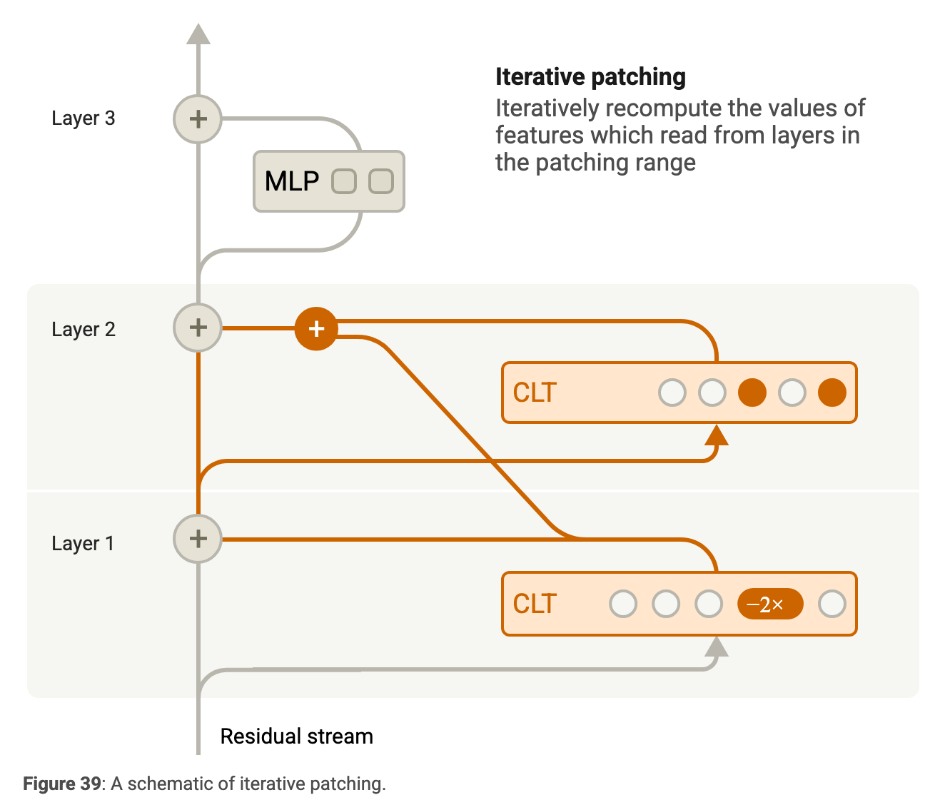
Iterative patching recomputes features within the patching range, allowing knock-on effects and newly activated units. Repeated encoding and decoding can amplify errors, making constrained patching easier to interpret for specific edge tests.
Details of Interventions
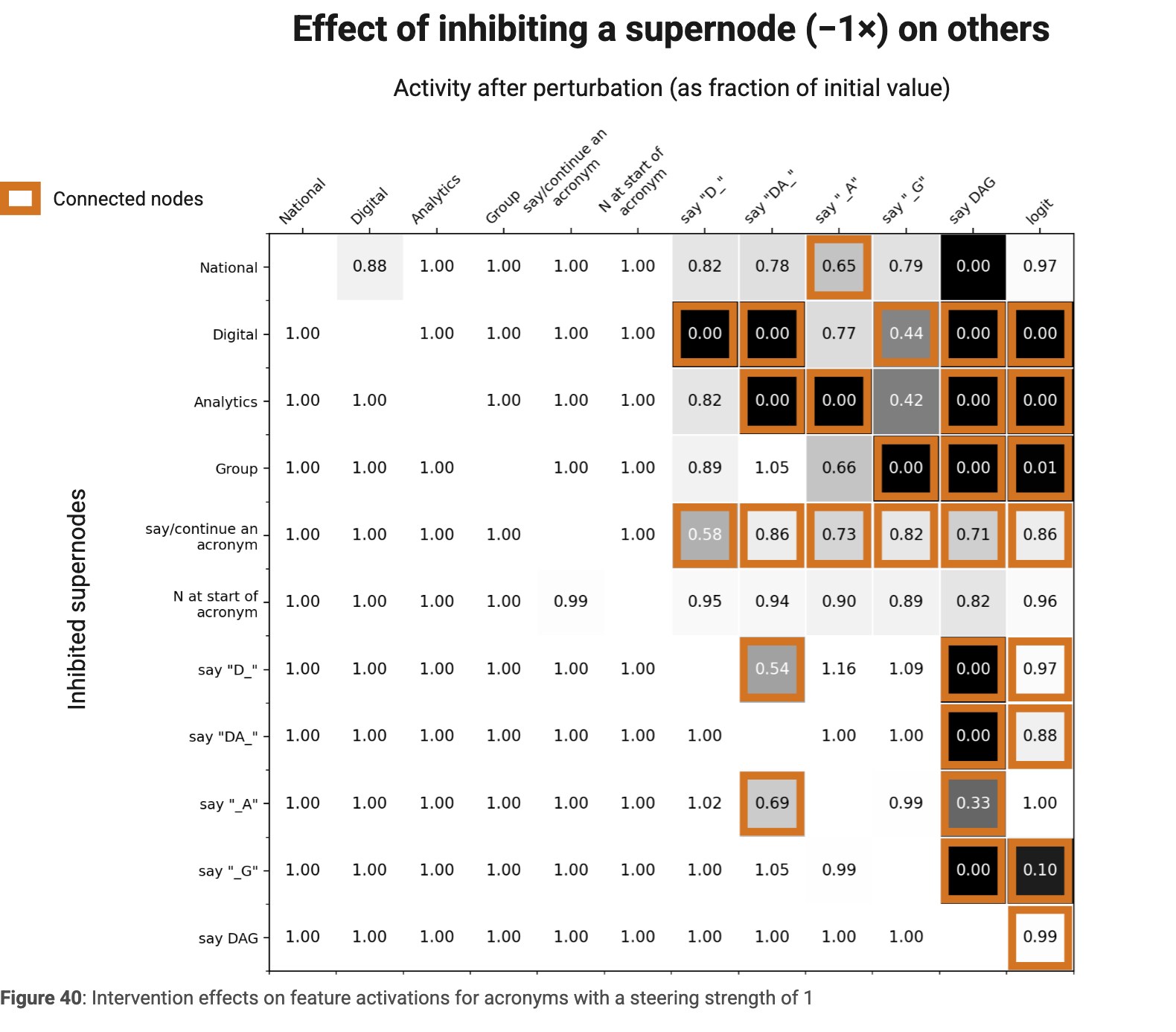
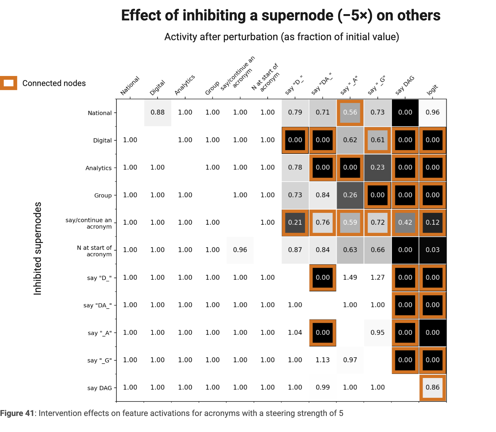
Full intervention plots show that different supernodes require different strengths because they contain different numbers of features and have different direct or indirect output connections.
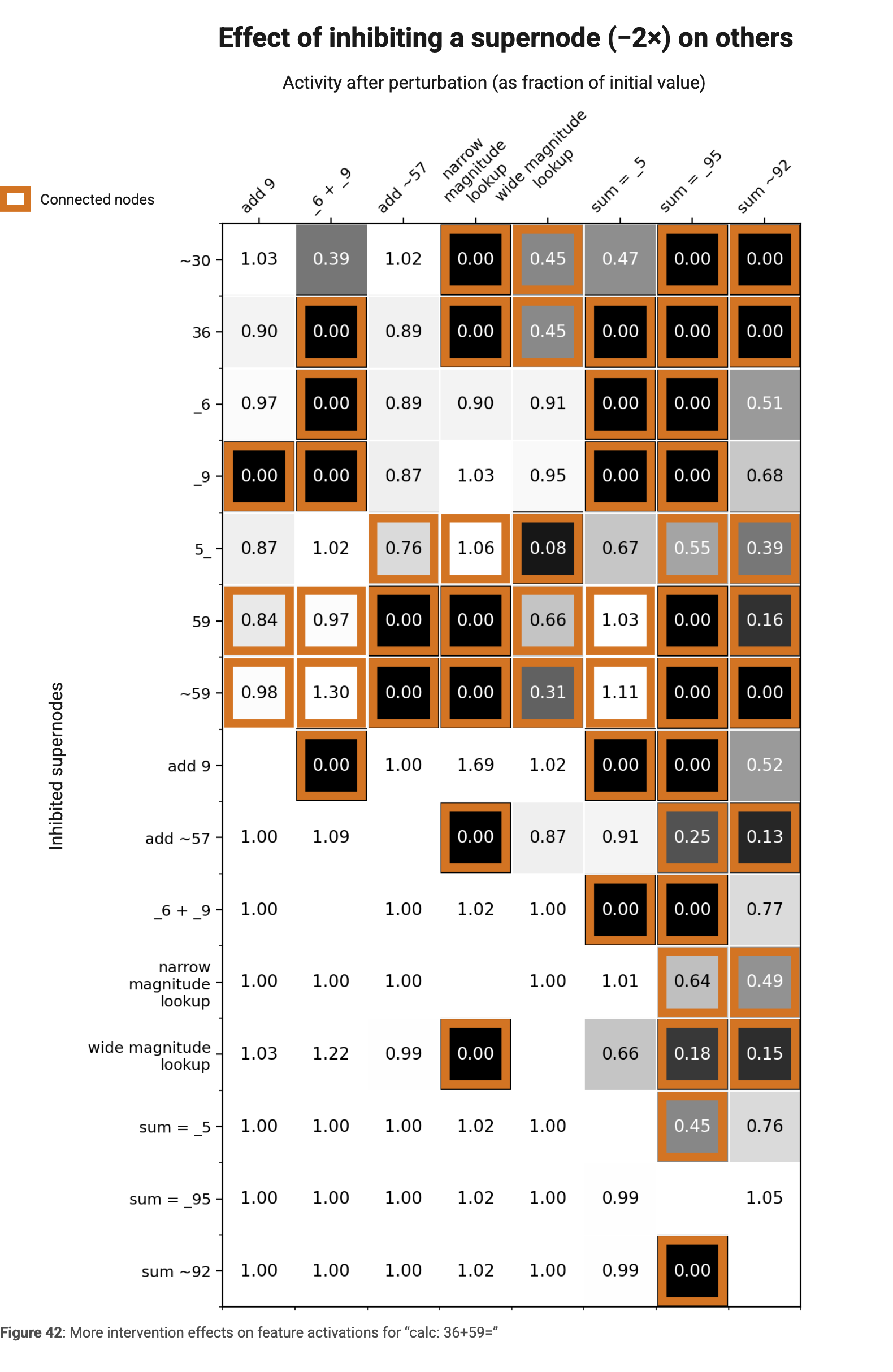
Notes on the Interface
The public graph interface is available under the MIT license. The internal version additionally supports feature scatterplots, labeling, richer hover information, graph differences, and rearrangeable analysis panels.
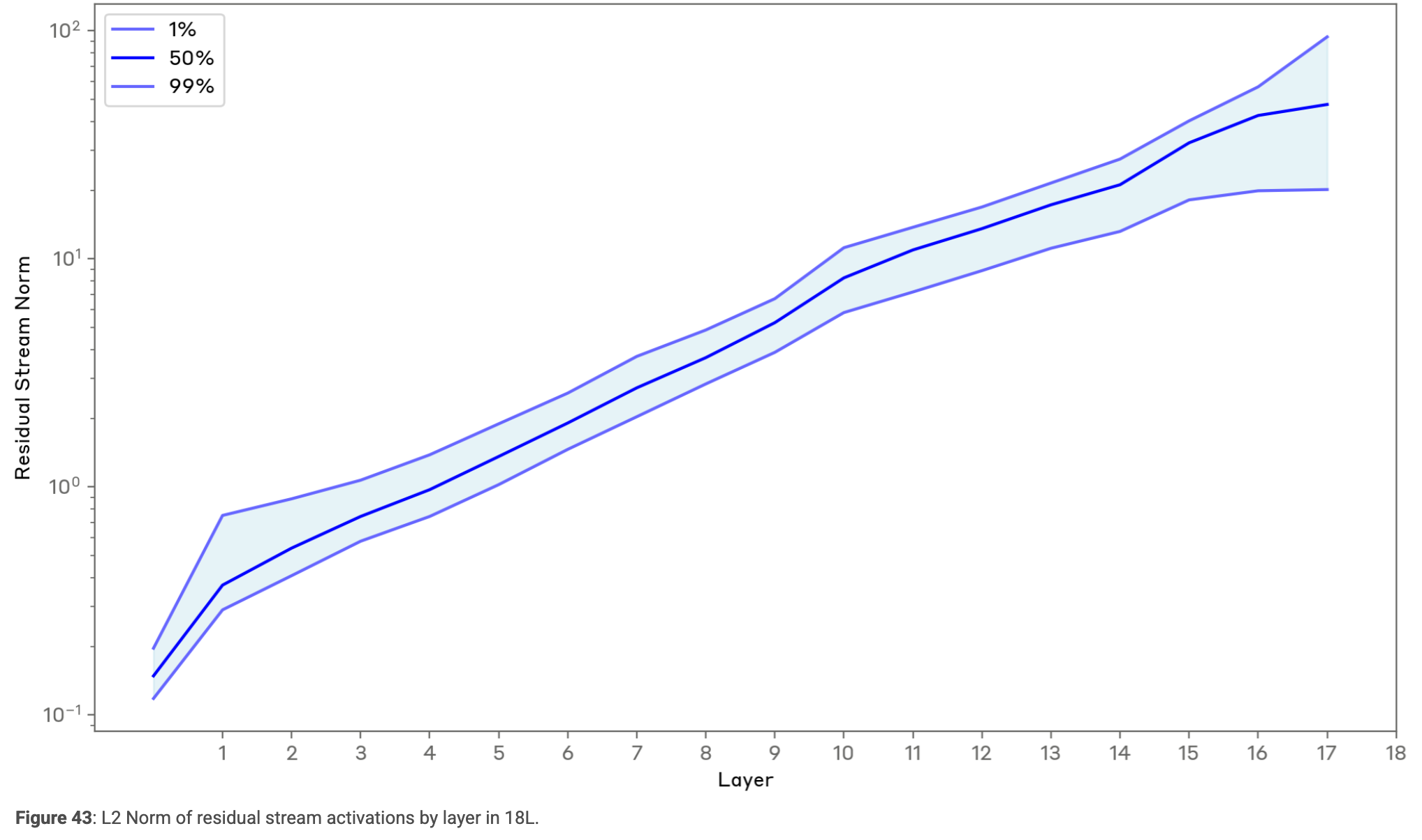
Residual Stream Norms Growth
Residual-stream norm growth can require repeated amplification to keep old information influential. A CLT can collapse this multilayer process into one feature, simplifying graphs while changing their apparent depth.
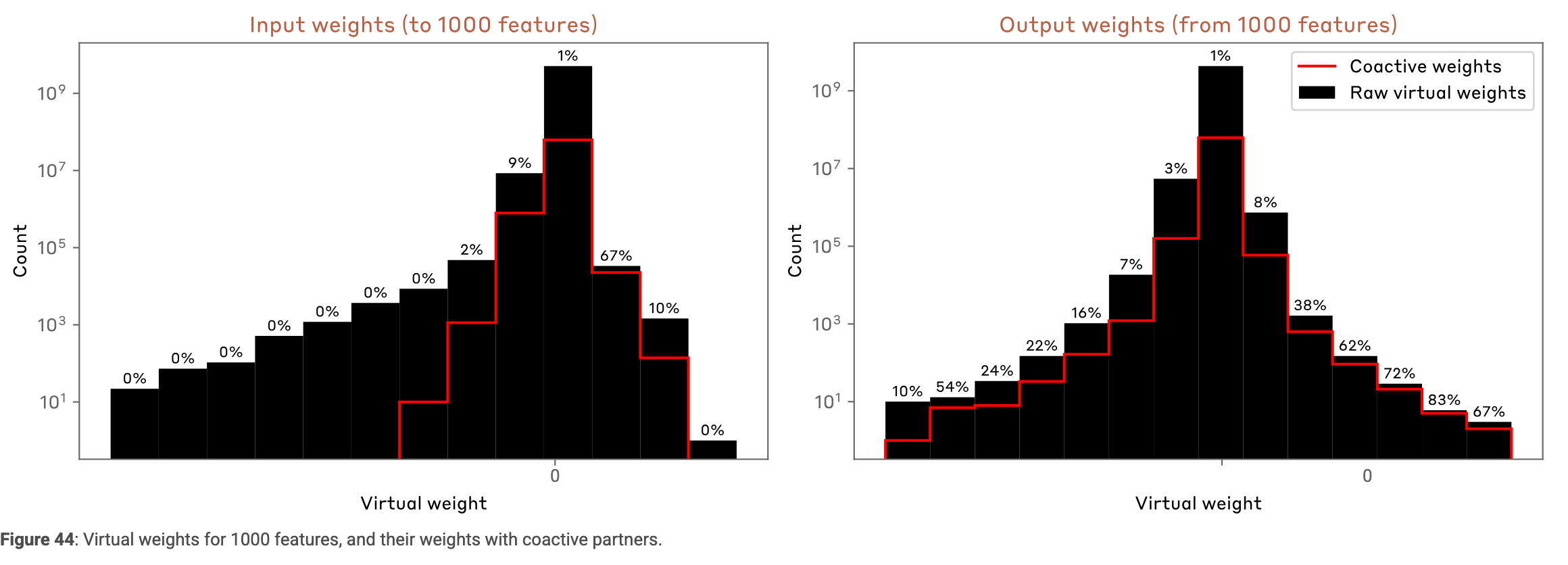
Interference Weights over More Features
Across one thousand arithmetic-related features and roughly 150 million tokens, many large virtual weights connect features that never coactivate. This suggests interference but is not conclusive: rare relevant contexts may be missed, and inhibitory weights can themselves prevent coactivation.
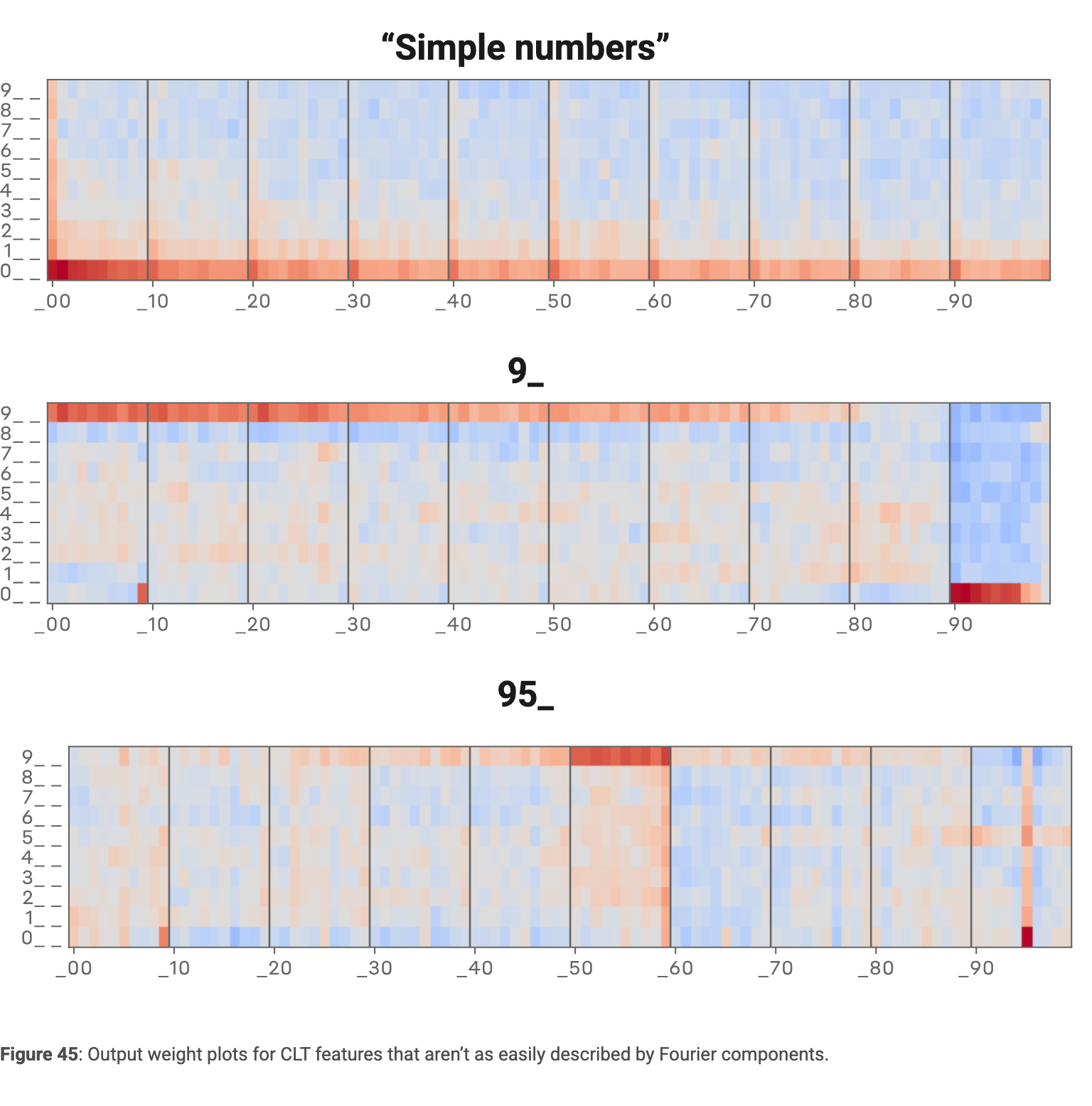
Number Output Weights for Select Features
The retained plots show complete output-token weights for features favoring simple numbers and numbers beginning with particular digits, including behavior outside the usual zero-to-ninety-nine display range.
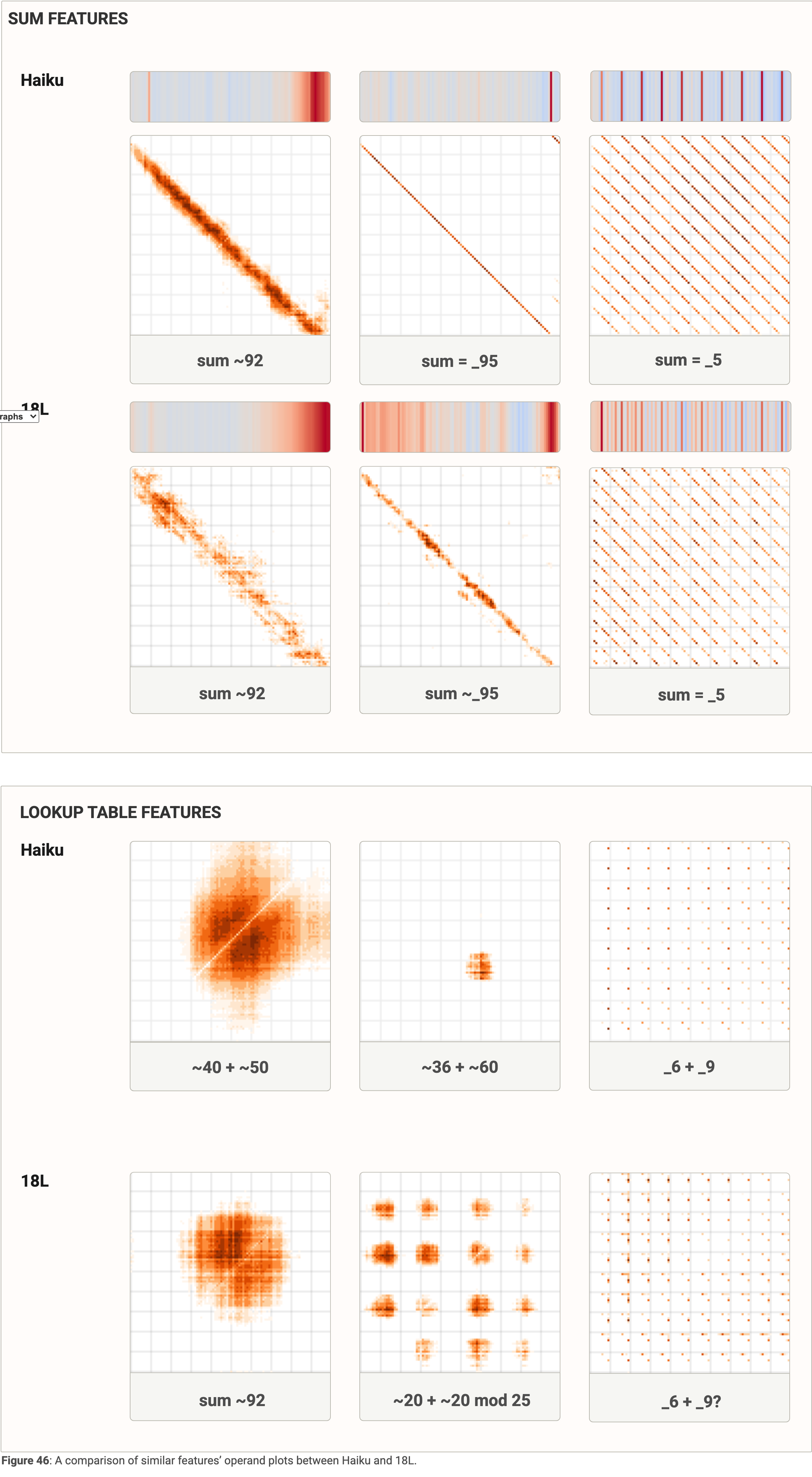
Comparison of Addition Features Between Small and Large Models
Both models exhibit similar addition-feature families, but the smaller model’s features are less precise. On the studied prompts it achieves 98.6% top-choice accuracy, compared with 100% for Haiku.
Additional Evaluation Details
The graph evaluation uses 260 selected nontrivial pretraining examples: correct predictions, uncommon target tokens, no repeated target in context, and a loss threshold excluding especially easy continuations. Results should not be interpreted as an unrestricted deployment sample.
Prompt and Graph Lists
The retained tables link to graphs for sampled pretraining prompts and curated recall, analogy, arithmetic, multilingual, memorization, and in-context-learning examples. Source footnotes clarify the modeling assumptions and evaluation choices discussed above.
Links | Prompt | Target |
|
| |
|
| |
|
| |
|
| |
|
|
Links | Prompt | Target |
|
| |
|
| |
|
| |
|
| |
|
| |
|
| |
|
| |
|
| |
|
| |
|
| |
|
| |
|
| |
|
| |
|
| |
|
| |
|
|