Overview
Intuition. Treat a neural activation vector like a recording containing several instruments. Individual coordinates mix contributions, so inspecting one coordinate may be confusing. Dictionary learning instead asks which few reusable patterns, drawn from a larger menu, can explain the whole vector.
Reading the math. Write x ≈ Da: x is the observed activation, columns of D are learned feature patterns, and a gives their strengths. A reconstruction loss keeps Da close to x; a sparsity penalty encourages only a few strengths to be nonzero. The encoder predicts those strengths. An accurate reconstruction does not by itself prove that each pattern has one clean meaning; the paper also examines examples and interventions.
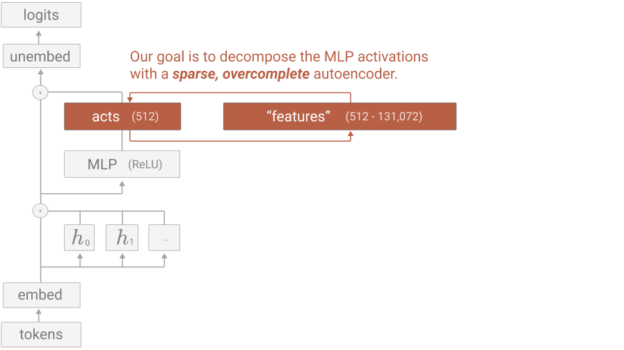
Sparse autoencoders decompose a one-layer transformer’s 512-neuron MLP into many more, comparatively interpretable features. Training uses over eight billion activation samples; the principal analysis studies 4,096 features. Case studies, human ratings, automated explanations, and interventions support their usefulness, without showing that every feature is pure or the model fully understood. [5] [17]
Summary of Results
Learned features can be more specific than neurons, have predictable causal effects, recur across independently initialized models, and subdivide as dictionaries grow. The largest dictionary contains 131,072 elements. Some features interact through generated tokens in patterns resembling finite-state machines.
Problem Setup
The testbed is a one-layer ReLU transformer trained on 100 billion Pile tokens. Sparse autoencoders reconstruct its 512-dimensional MLP activations using 512–131,072 dictionary elements. This simple model makes output effects comparatively easy to inspect; larger-model generalization is a separate question.
Transformer | Sparse Autoencoder | |
Layers | 1 ReLU (up) | |
MLP Size | 512 | 512 (1×) – 131,072 (256×) |
Dataset | The Pile[19] | Transformer MLP Activations |
Loss | Autoregressive Log-Likelihood |
Features as a Decomposition
An activation vector is approximated by a bias plus a weighted sum of unit feature directions. A ReLU encoder estimates the nonnegative weights; decoder columns provide the directions. The decomposition is a sparse matrix factorization, and the authors remain agnostic about whether it uniquely identifies the model’s fundamental components.
Equations
Superposition Hypothesis
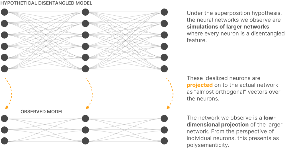
The superposition hypothesis motivates an overcomplete dictionary: many sparse features may share a lower-dimensional activation space with tolerable interference. Sparsity is what makes recovery plausible despite having more candidate features than neurons.
What makes a good decomposition?
A useful decomposition should explain when features activate, predict the effects of changing them, and preserve substantial model functionality. Those properties support monitoring and intervention, but identifying components is only a first step toward understanding their interactions.
Why not use architectural approaches?
Enforcing sparse neuron activity does not guarantee semantic purity. A simple cross-entropy example achieves lower loss by grouping mutually exclusive categories in one neuron than by representing only one category precisely. The authors therefore favor post-training decomposition; their conclusion about architectural approaches is motivated by counterexamples rather than a universal impossibility theorem.
Using Sparse Autoencoders To Find Good Decompositions
Exact sparse recovery can be computationally difficult. The authors choose a single-layer sparse autoencoder because it scales to billions of examples and has a decoding capacity comparable to the transformer MLP, rather than relying on a much stronger iterative solver.
Sparse Autoencoder Setup
The autoencoder subtracts its decoder bias, applies an independently parameterized linear encoder and ReLU, then reconstructs with a linear decoder. Adam minimizes reconstruction error plus an L1 activation penalty. Large datasets and periodic resampling of dead features substantially improve the authors’ practical results.
How can we tell if the autoencoder is working?
No single reliable quality metric emerged. The study combines manual inspection, feature-density distributions, reconstruction loss, and toy problems with known ground truth. A candidate information-based objective did not consistently track interpretable or suitably sparse solutions.
The (one-layer) model we're studying
Two transformers share architecture, hyperparameters, and training data but differ in initialization. Dictionaries A and B use different activation samples. The one-layer setup makes approximate logit effects easy to calculate, while its simplicity limits conclusions about deeper models.
Notation for Features
Identifiers such as A/1/2357 specify transformer A, dictionary run 1, and feature 2357. A/0 through A/5 increase dictionary size at a fixed sparsity coefficient. The separate “neurons” identifier refers to an original transformer unit.
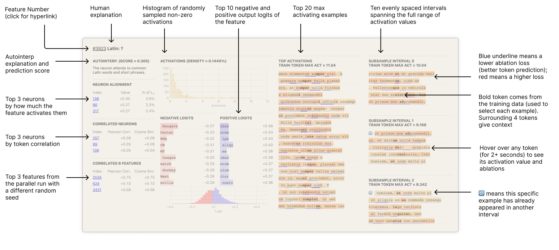
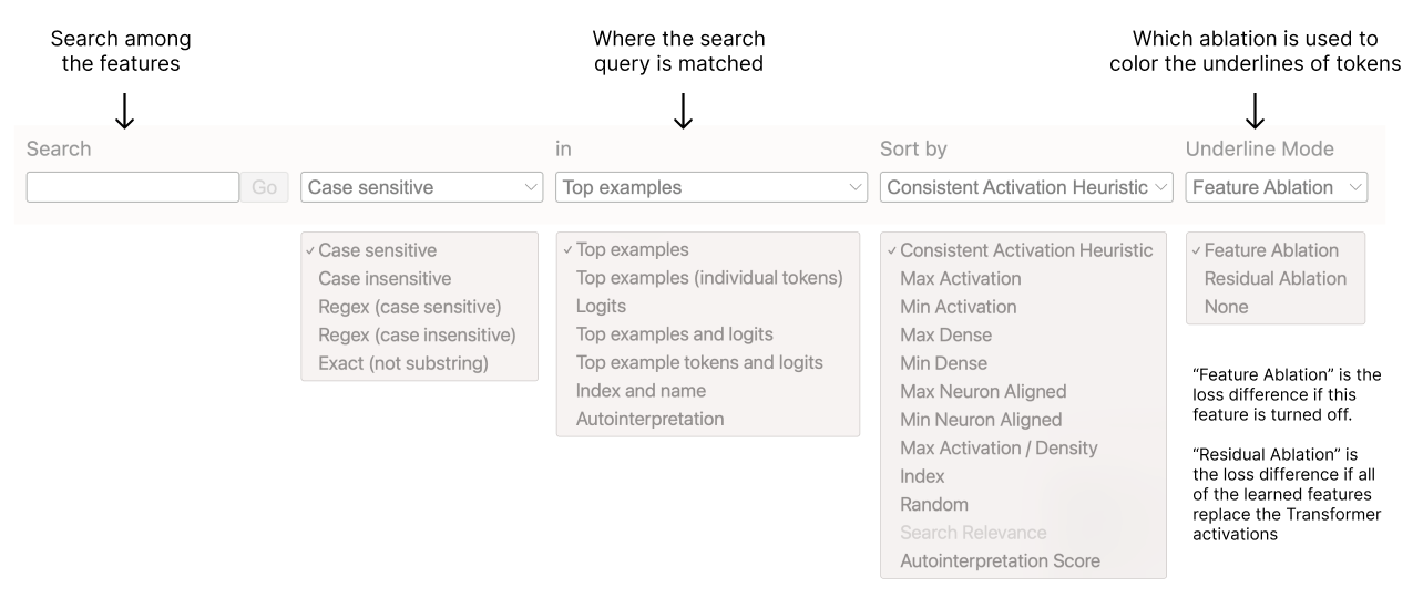
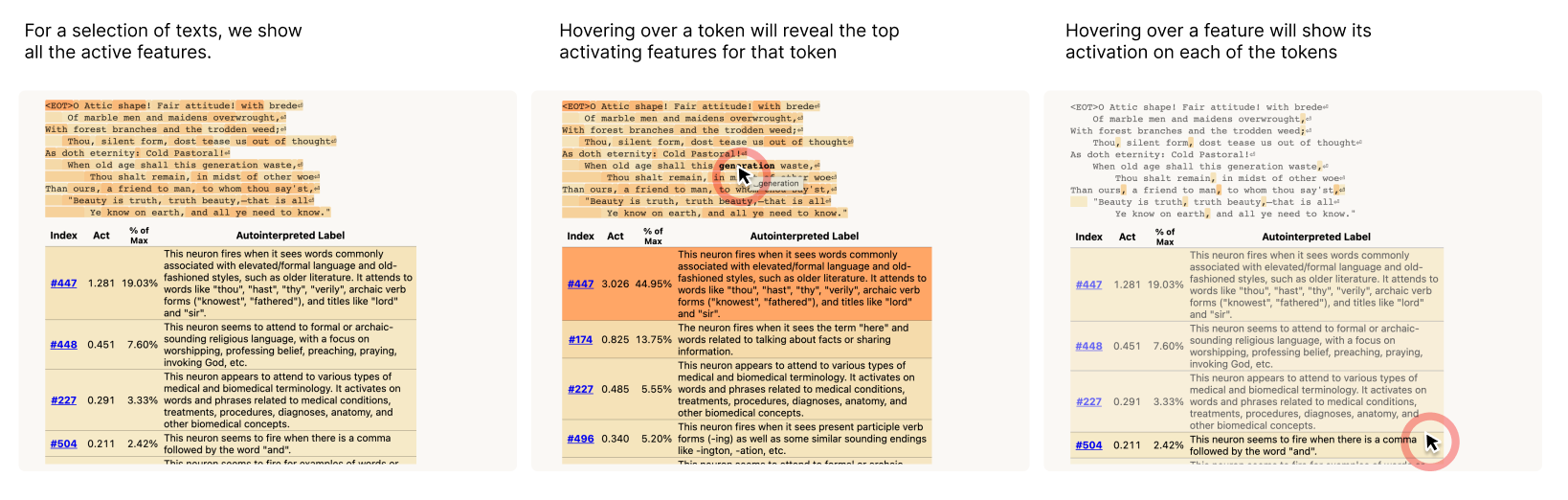
Interface for Exploring Features
The companion explorer provides activating examples, output-logit effects, ablations, search, and views of all features active on selected texts. The retained interface illustrations link back to the original interactive resource.
Detailed Investigations of Individual Features
Four deliberately tractable case studies examine Arabic script, DNA, base64, and Hebrew script. Character-based likelihood proxies test specificity and sensitivity; output effects, ablations, neuron comparisons, and a second model test functional relevance. These examples are selected for ease of analysis, so broader claims require the later population evaluations.
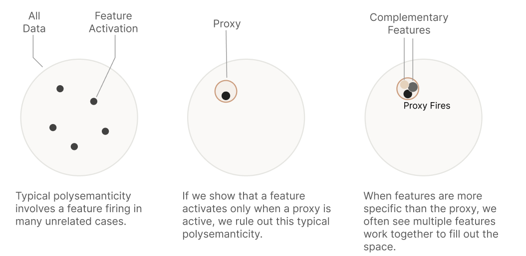
Arabic Script Feature
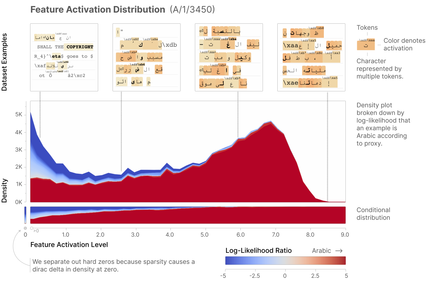
Feature A/1/3450 responds to Arabic script across languages including Arabic, Farsi, and Urdu. Its behavior is much more specific than that of any individual neuron inspected.
Activation Specificity
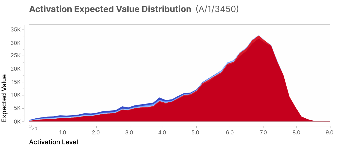
Arabic-script tokens form 0.13% of the dataset but 81% of this feature’s nonzero activations. Specificity rises from 25% at very weak activation to 98% above activation five. Tokenization, shared punctuation, imperfect confidence, and reconstruction error can all explain some apparent low-activation exceptions.
Activation Sensitivity
Other features cover the Arabic definite article and different bytes of split Unicode characters. The main feature’s activation correlates 0.74 with the thresholded script proxy across roughly 40 million tokens; no single Arabic feature covers every relevant token.
Feature Downstream Effects
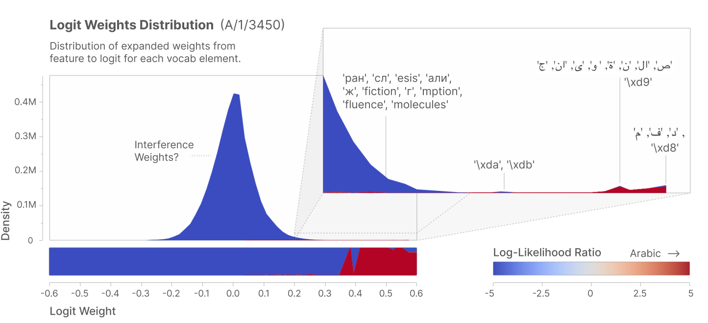
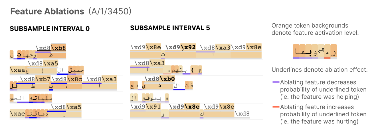
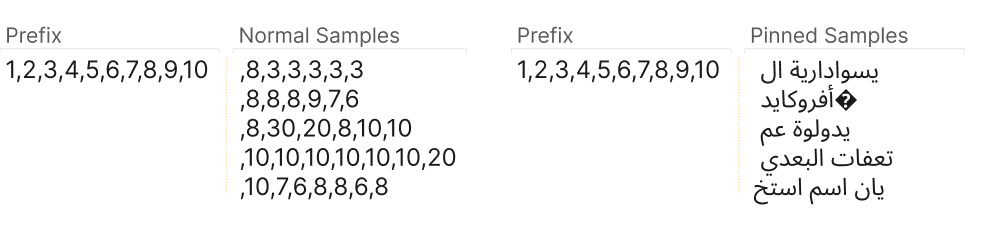
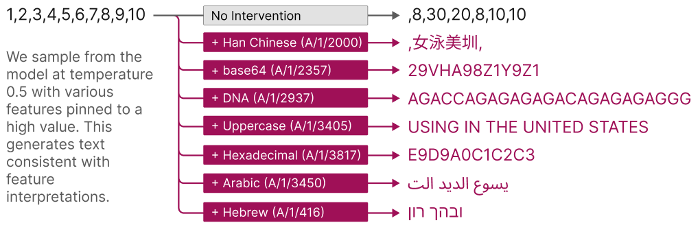
Approximate logit weights favor Arabic-script continuations. Subtracting this feature from actual MLP activations reduces appropriate token predictions, and pinning it high steers generation toward Arabic. These tests use model outputs that were not part of the autoencoder training objective.
The feature is not a neuron
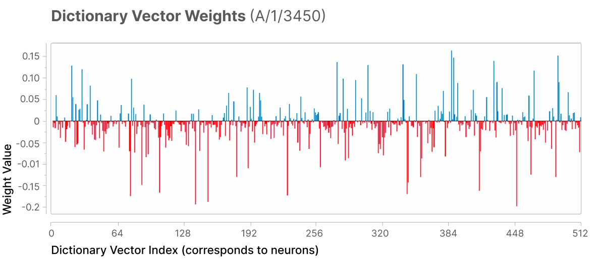
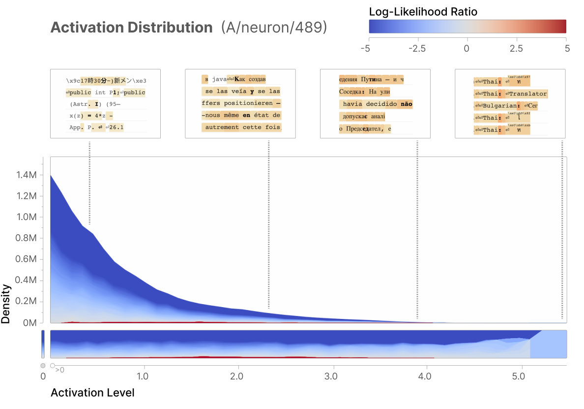
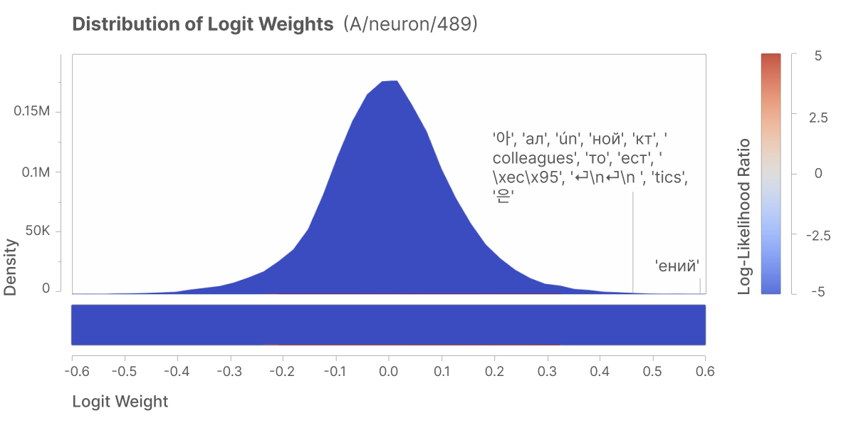
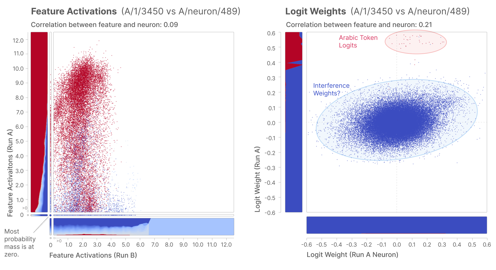
The Arabic direction is distributed across many neurons, including substantial negative coefficients. Its most correlated neuron responds to several languages and has much less specific output effects. Inspecting top neuron activations would largely miss this feature.
Universality
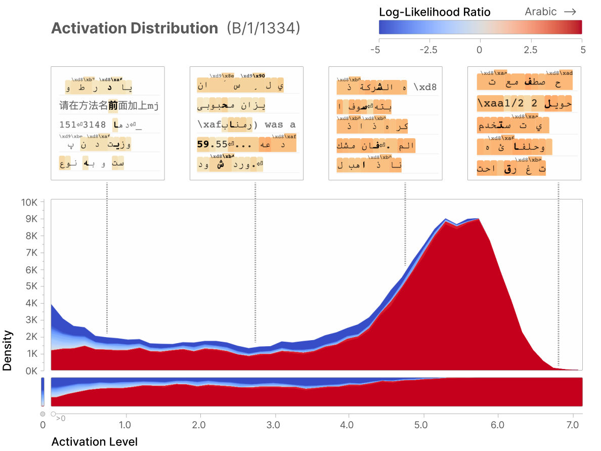
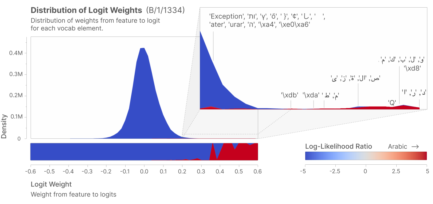
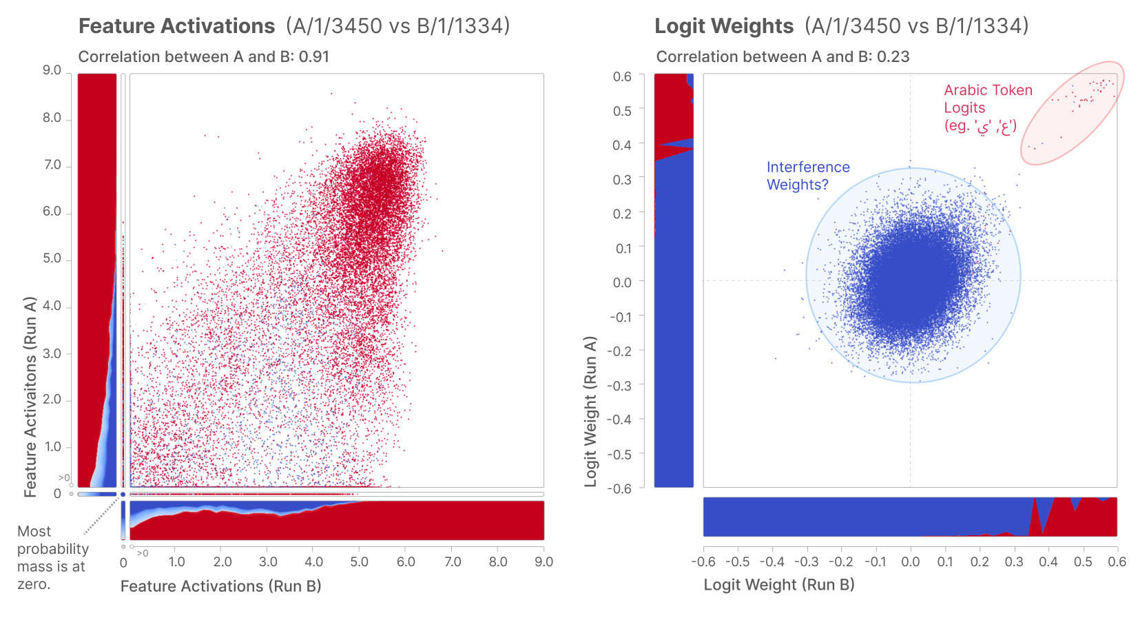
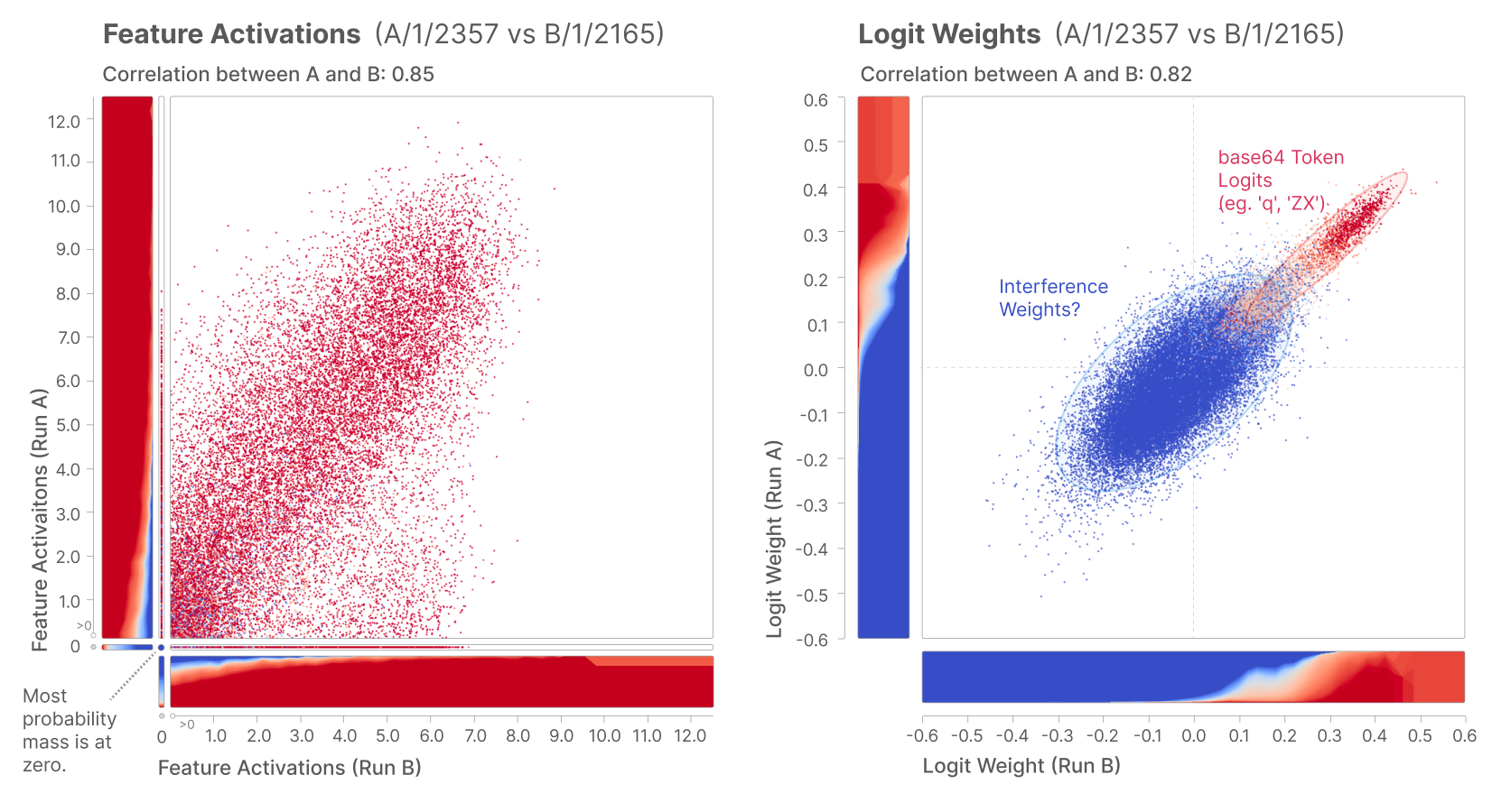
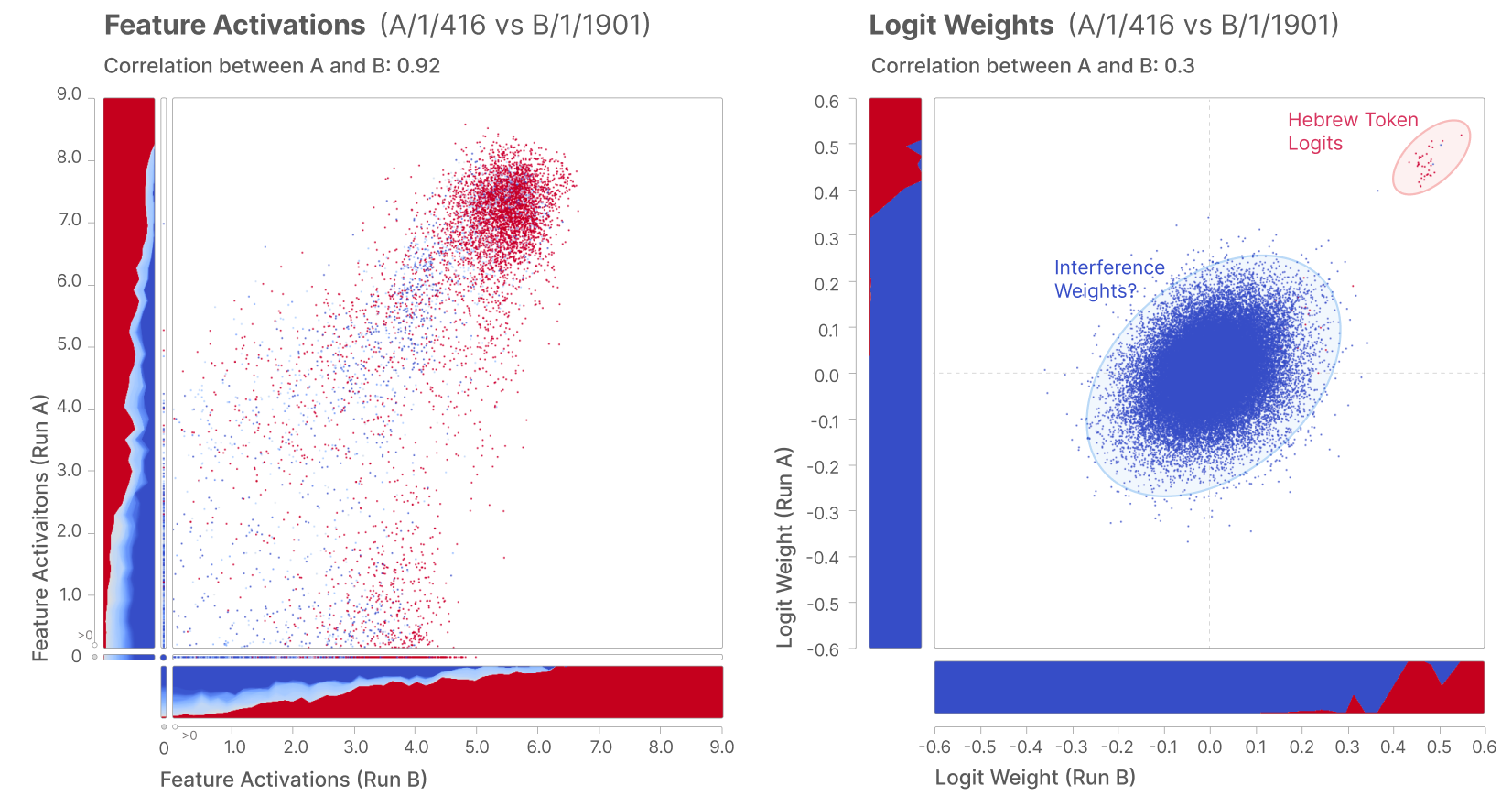
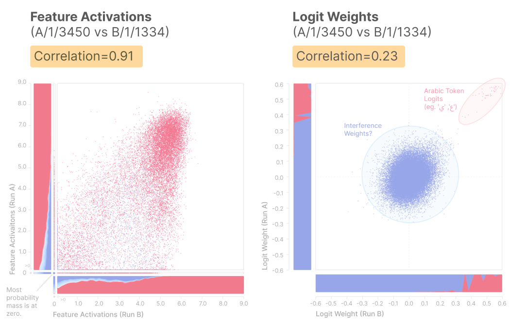
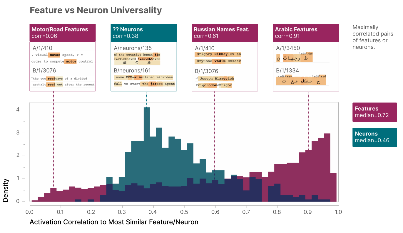
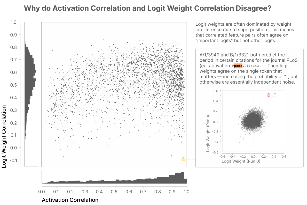
The independently initialized B model contains a matching Arabic feature with activation correlation 0.91. Their strongly upweighted Arabic tokens agree more clearly than the numerous small output weights, which the authors interpret as possible interference.
DNA Feature
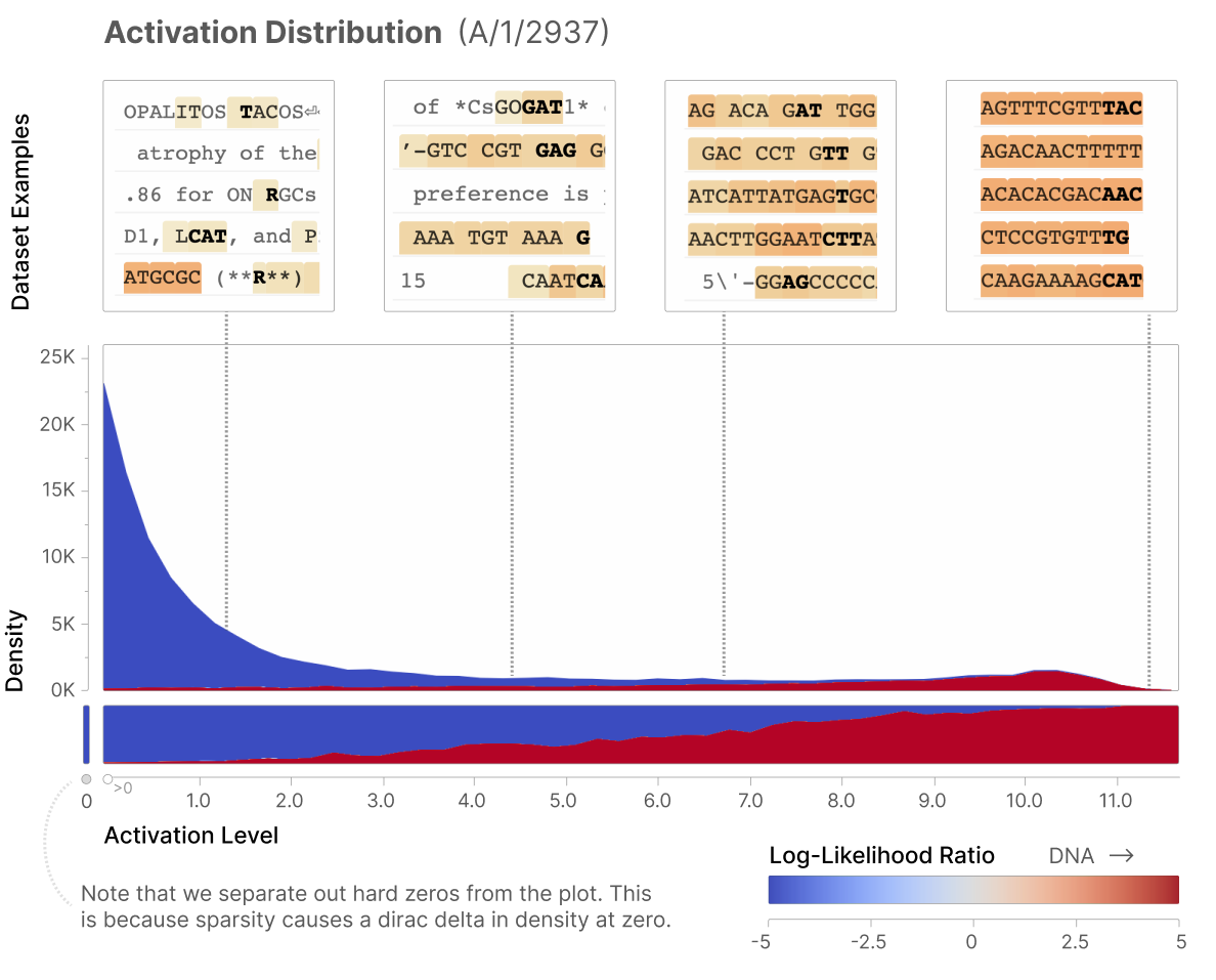
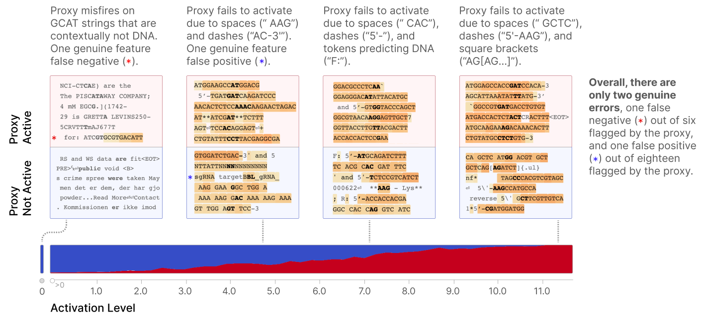
Feature A/1/2937 responds to nucleotide sequences. Unlike Arabic, this context is largely captured by one feature in the principal dictionary. Its behavior includes some valid sequence formatting that the strict character proxy misses.
Activation Specificity and Sensitivity
The thresholded DNA proxy correlates 0.80 with feature activity. Inspection finds many proxy disagreements are genuine sequences containing spaces, punctuation, or missing-base notation. The feature can start after the first few sequence tokens, and high activations are particularly specific.
Feature Downstream Effect
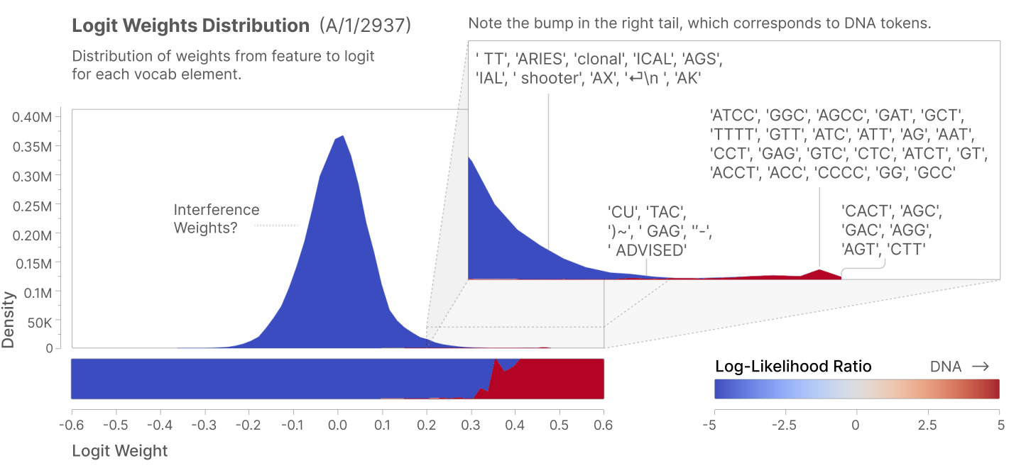
The DNA feature upweights combinations of nucleotide characters, consistent with continuing a sequence. These output effects independently support the activation-based interpretation.
The Feature Is Not A Neuron
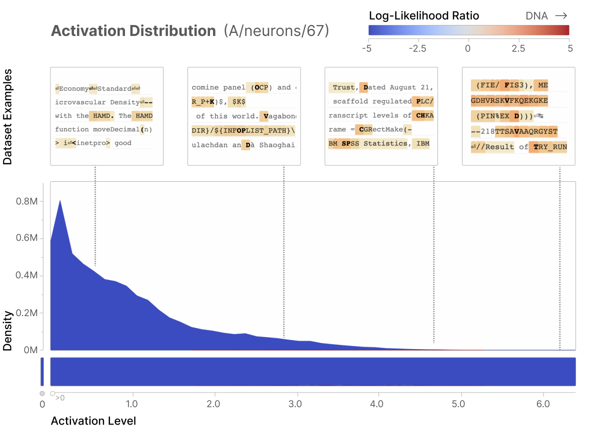
Neither the most activation-correlated neuron nor the neuron contributing most strongly to the dictionary direction has comparably specific DNA behavior. The learned feature is therefore not simply an already interpretable neuron.
Universality
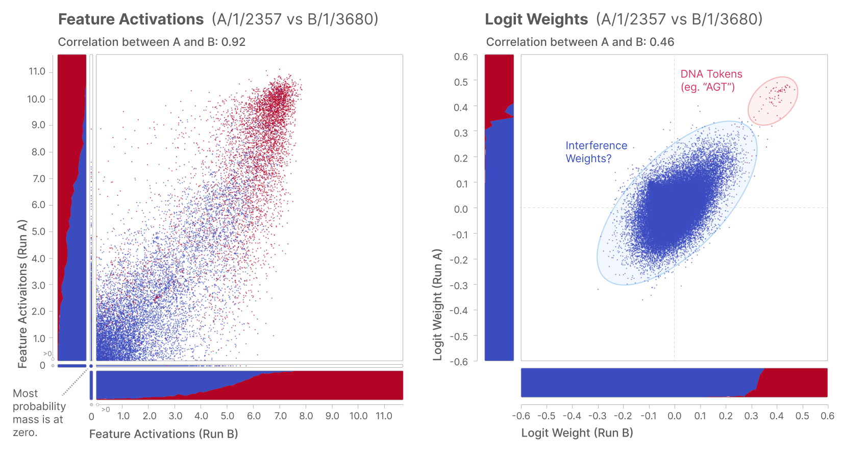
A matching feature in model B has activation correlation 0.92 and similar nucleotide-focused output weights. This supports reproducibility across the two matched model configurations.
Base64 Feature
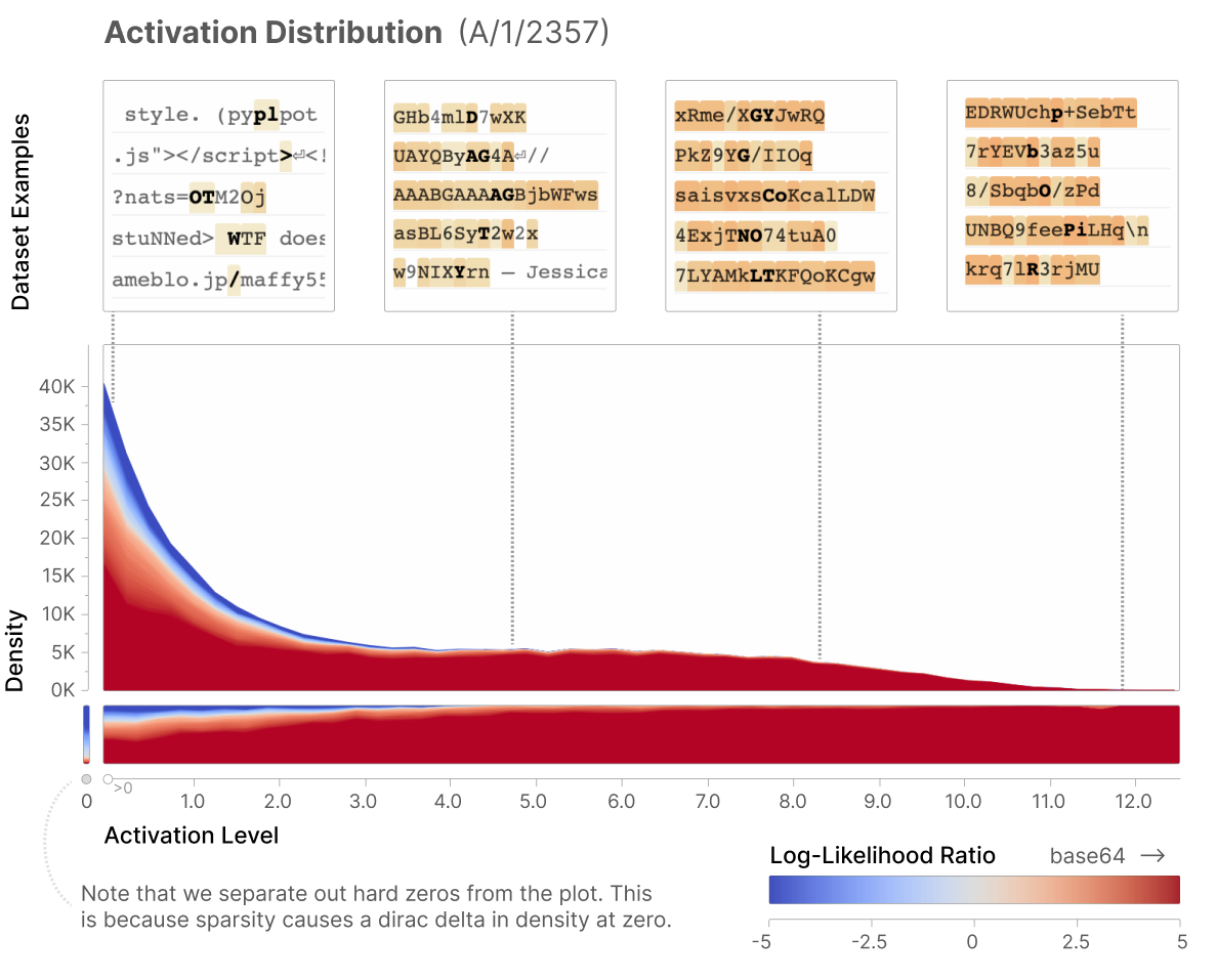
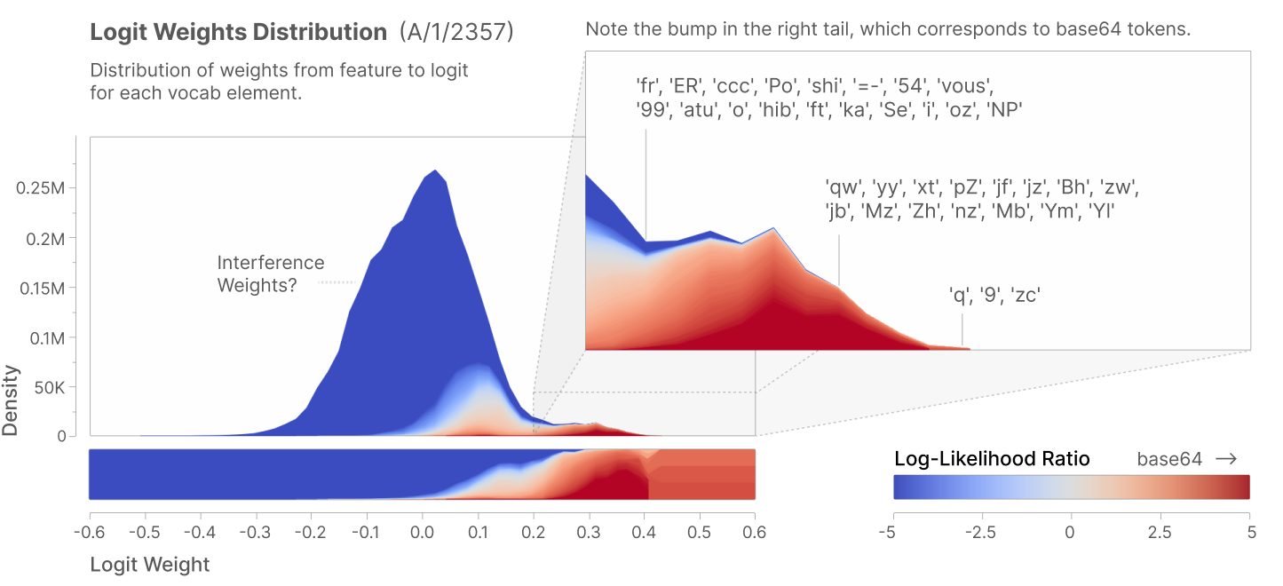
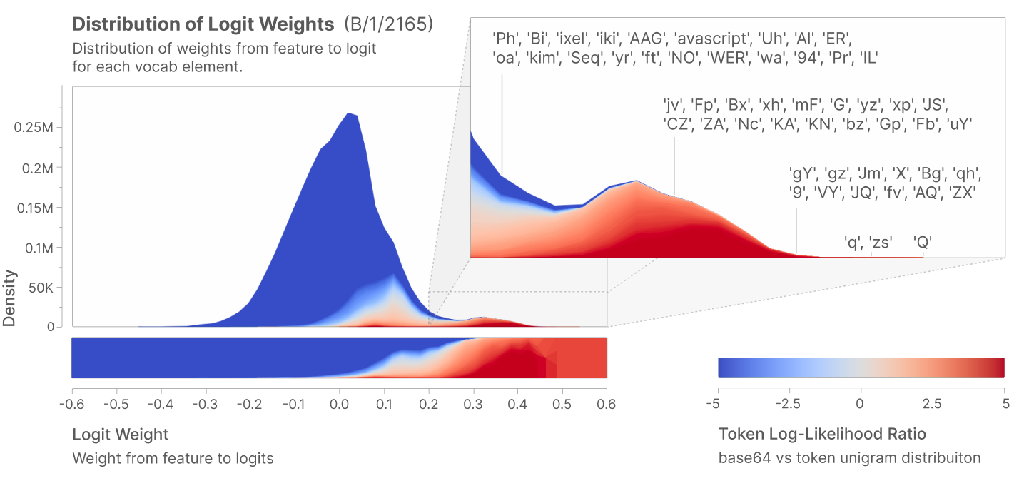
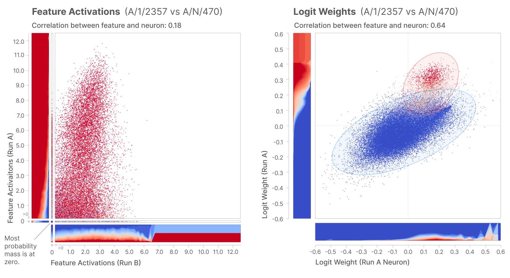
Feature A/1/2357 detects base64-like strings and favors corresponding continuations. Its proxy correlation is only 0.38 because the broad character proxy also detects contexts such as hexadecimal strings, which have their own features. Additional base64 features handle important subcases.
Universality
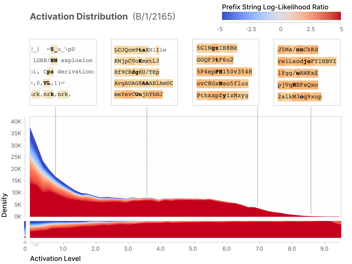
The closest base64 feature in model B has activation correlation 0.85 and similar output preferences. Tokens shared with ordinary language make the boundary between base64-specific and background logit weights less sharp.
The Feature Is Not A Neuron
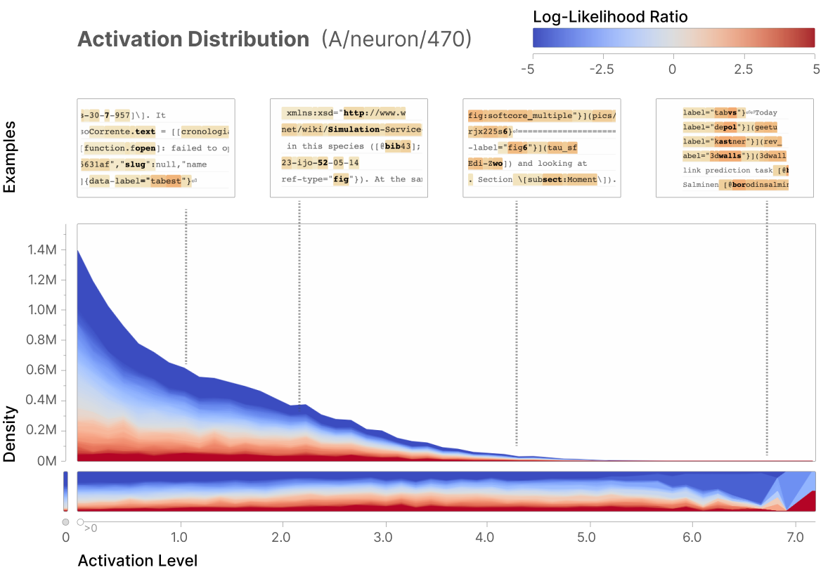
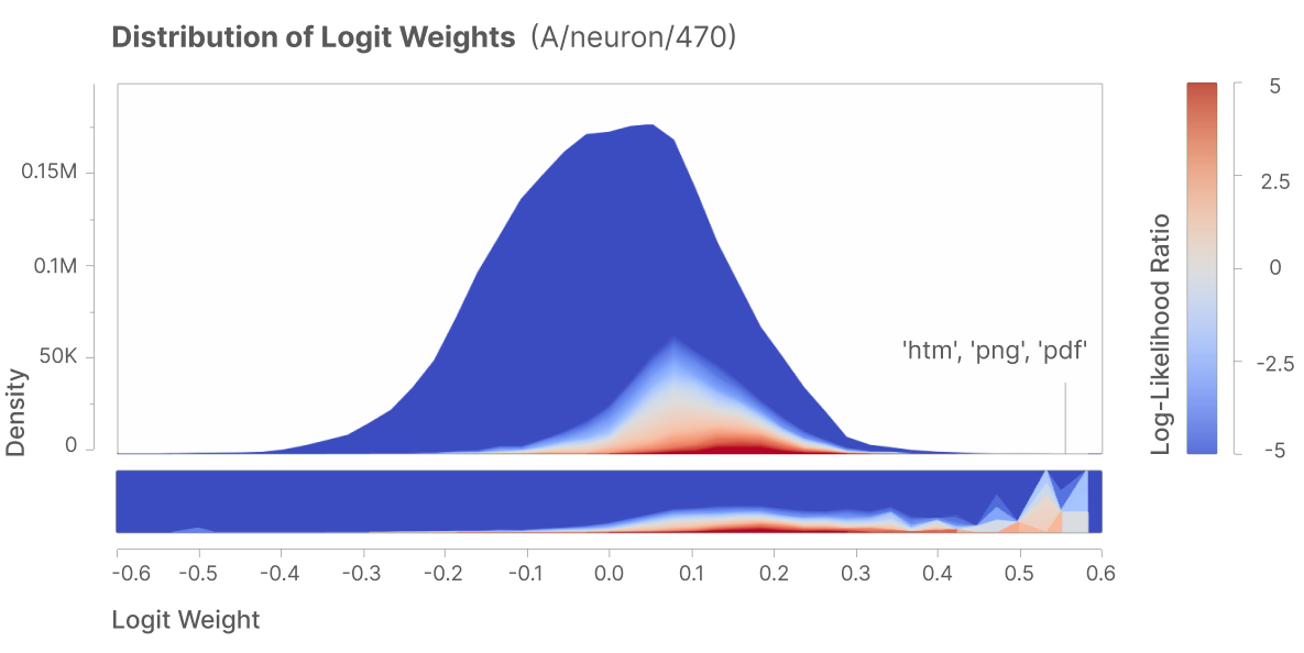
The closest original neuron correlates only 0.18 with the base64 feature and also responds to code, markup, and URL fragments. Its output effects are correspondingly mixed.
Hebrew Feature
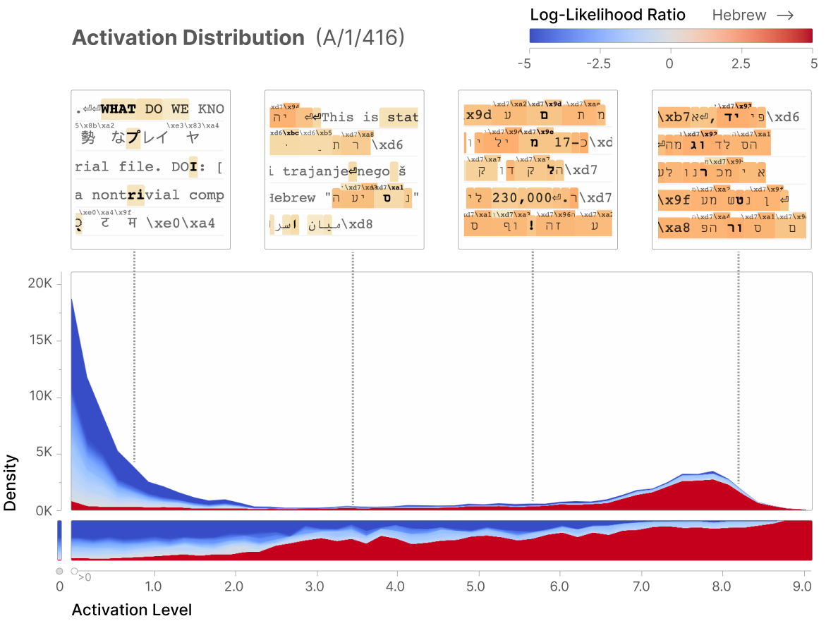
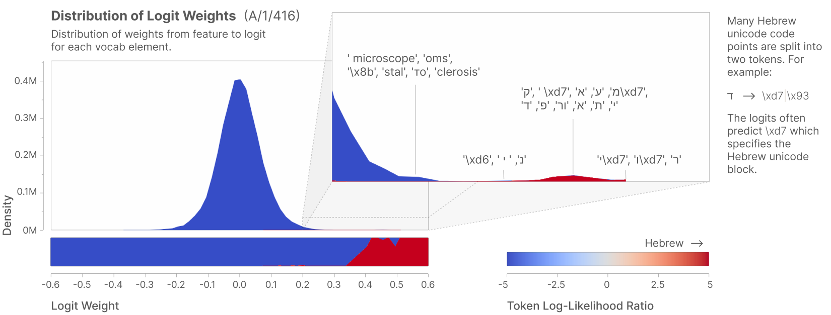
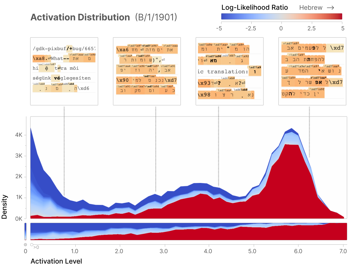
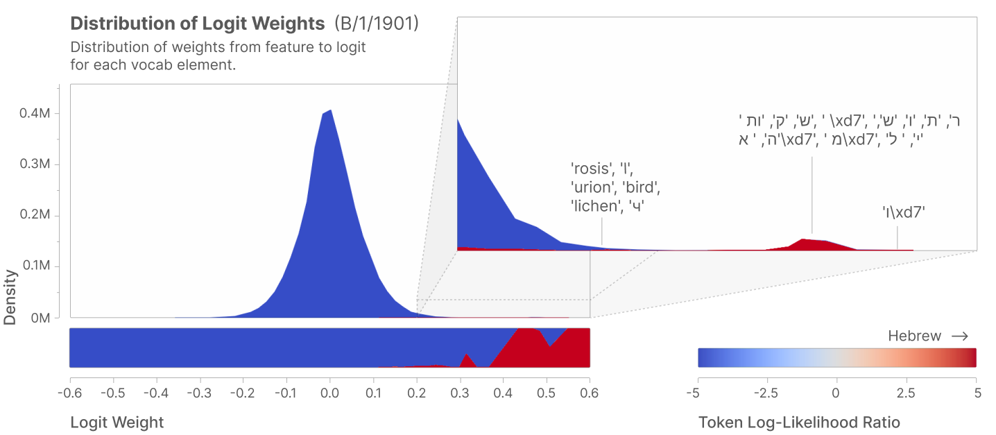
Feature A/1/416 strongly responds to Hebrew script and upweights Hebrew continuations. Proxy correlation is 0.55; common punctuation and complementary features for incomplete Unicode characters explain some gaps. Weak activations are less specific.
The Feature Is Not A Neuron
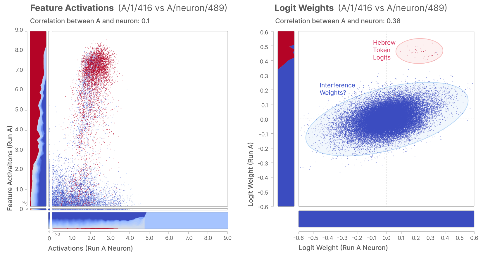
The closest neuron has activation correlation only 0.10 and mixed language behavior. No neuron has basic Hebrew-block characters among its top dataset examples in the authors’ search.
Universality
Model B contains a Hebrew feature with activation correlation 0.92 and similar script-specific output weights. This parallels the other three selected contexts.
Global Analysis
Population analyses exclude 168 dead and 292 ultralow-density features from the 4,096-element principal dictionary. The remaining features are evaluated for interpretability and functional coverage; these exclusions matter when interpreting the reported typical-feature results.
How Interpretable is the Typical Feature?
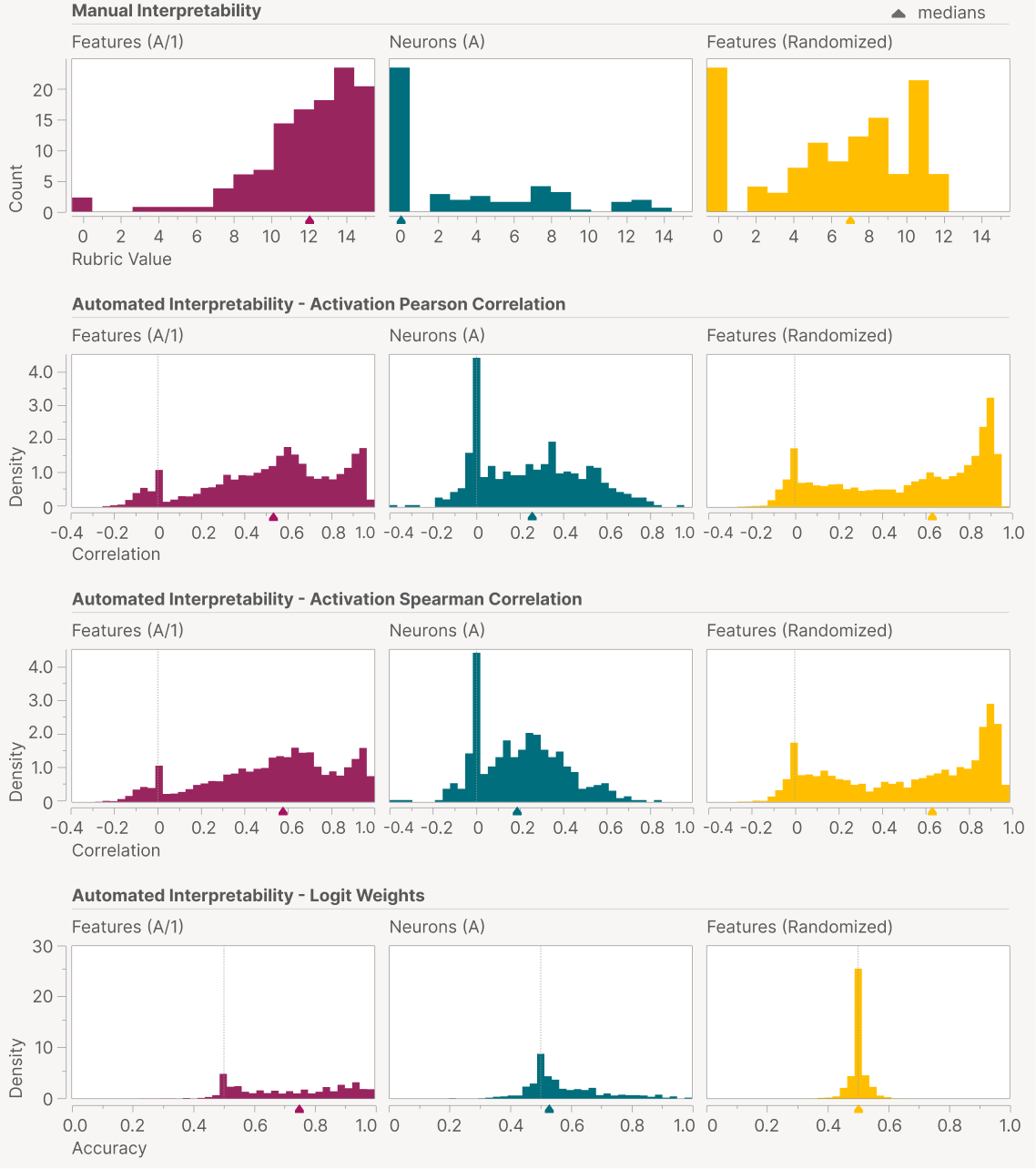
Three comparisons examine human judgments, language-model predictions of feature activity, and language-model predictions of output preferences. Each favors the learned features over original neurons, though they measure different aspects of interpretability.
Manual Human Analysis
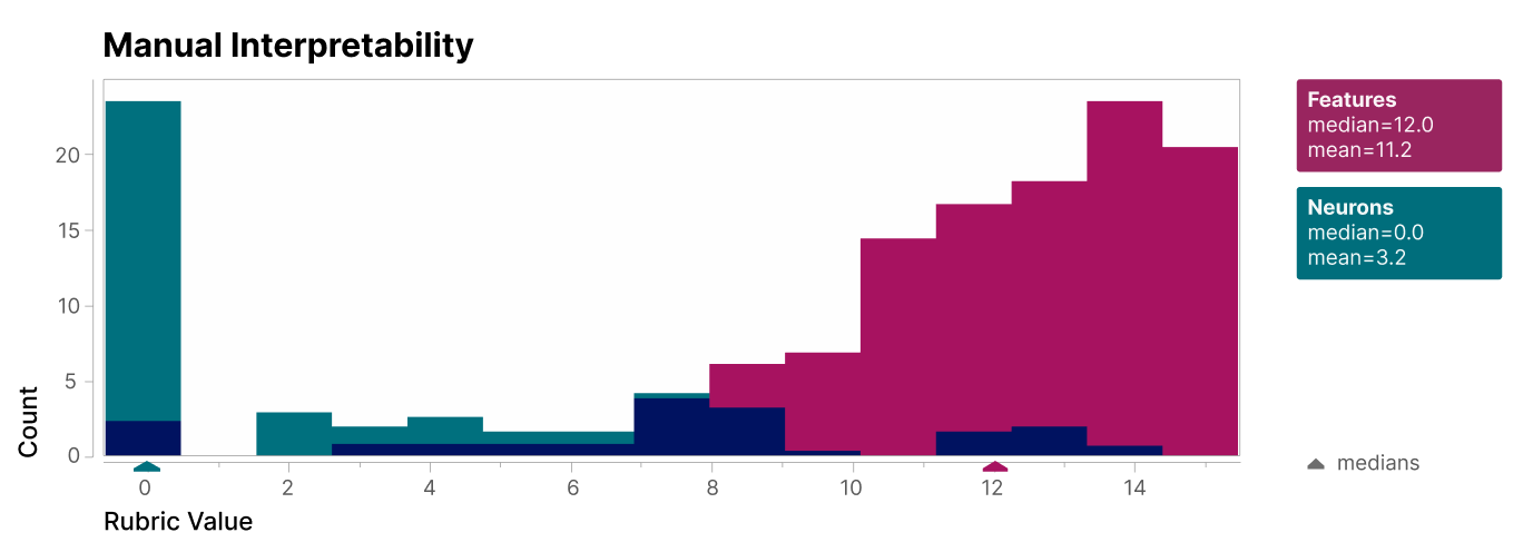
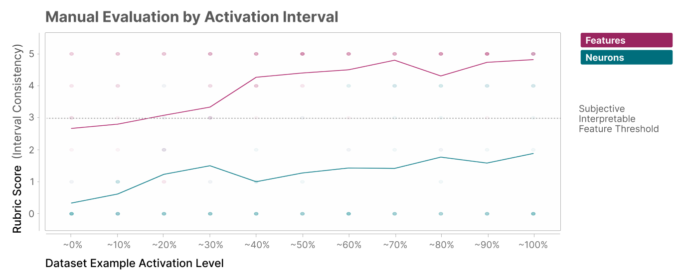
One blinded author rates 412 activation intervals across 162 features and neurons, including weak as well as strong activations. The median feature interval scores 12 versus zero for neurons under the paper’s rubric. This is a labor-intensive, single-annotator comparison rather than a broad human-consensus study.
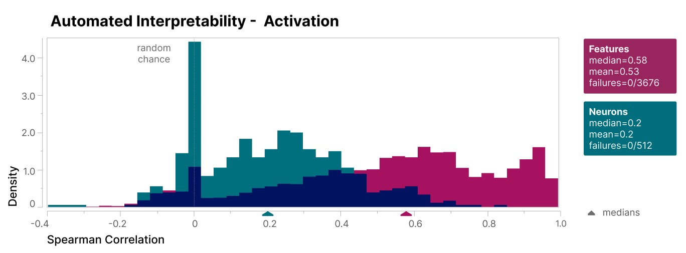
Automated Interpretability – Activations
Claude generates explanations and predicts held-out activations without seeing their true values. Spearman correlation over 60 nine-token examples per feature favors dictionary features. The sampling deliberately includes active intervals, and the appendix examines how reweighting changes the evaluation.
Automated Interpretability – Logit Weights
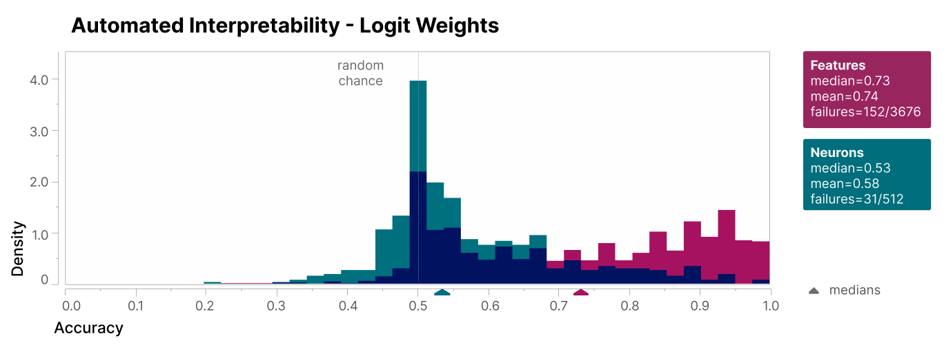
Using the same explanations, Claude distinguishes held-out strongly upweighted tokens from random tokens. Mean accuracy is 74% for features versus 58% for neurons, with a 50% chance baseline. This probes consistency between an interpretation and downstream effects.
Activation Interval Analysis
Higher-activation intervals generally fit the interpretations better. Some features remain consistent throughout their activity range; others become unclear below roughly the strongest 60%. Slightly misestimated directions are one possible explanation.
Caveats
Most nonzero activations are small and less interpretable, while larger activations can dominate output effects. Uniformly sampling features also differs from weighting them by functional importance. These issues limit any claim that the full activation distribution has been explained.
How much of the model does our interpretation explain?
Replacing the MLP with the principal autoencoder recovers 79% of its loss improvement over zero ablation; a 131,072-feature dictionary recovers 94.5%. These percentages measure functional reconstruction against that baseline, not the fraction of mechanisms understood or features discovered. Rare behavior and residual polysemanticity remain unresolved.
Do features tell us about the model or the data?
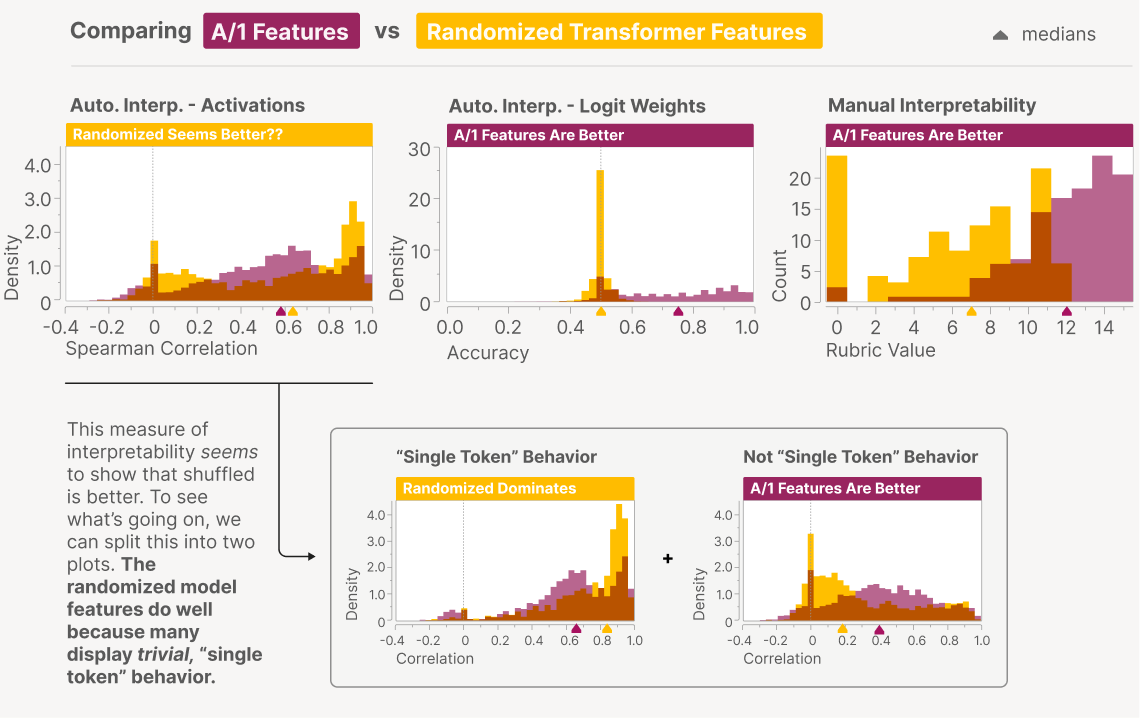
Dictionary learning on a weight-shuffled transformer mostly yields token detectors or hard-to-interpret mixtures. In the trained model, coherent logit effects, feature ablations, and pinned sampling support a relationship to learned computation rather than dataset correlations alone.
Phenomenology
The following observations describe feature families, comparisons across models, and interactions through generated text. They extend the empirical picture but do not establish a unique, exhaustive ontology of model features.
Feature Motifs
Common motifs include contexts, tokens within contexts, and longer phrase fragments. Because this is the last and only MLP, a feature can be interpreted both by what activates it and by which continuation it promotes. Larger dictionaries expose many distinct context-sensitive uses of the same token.
Feature Splitting
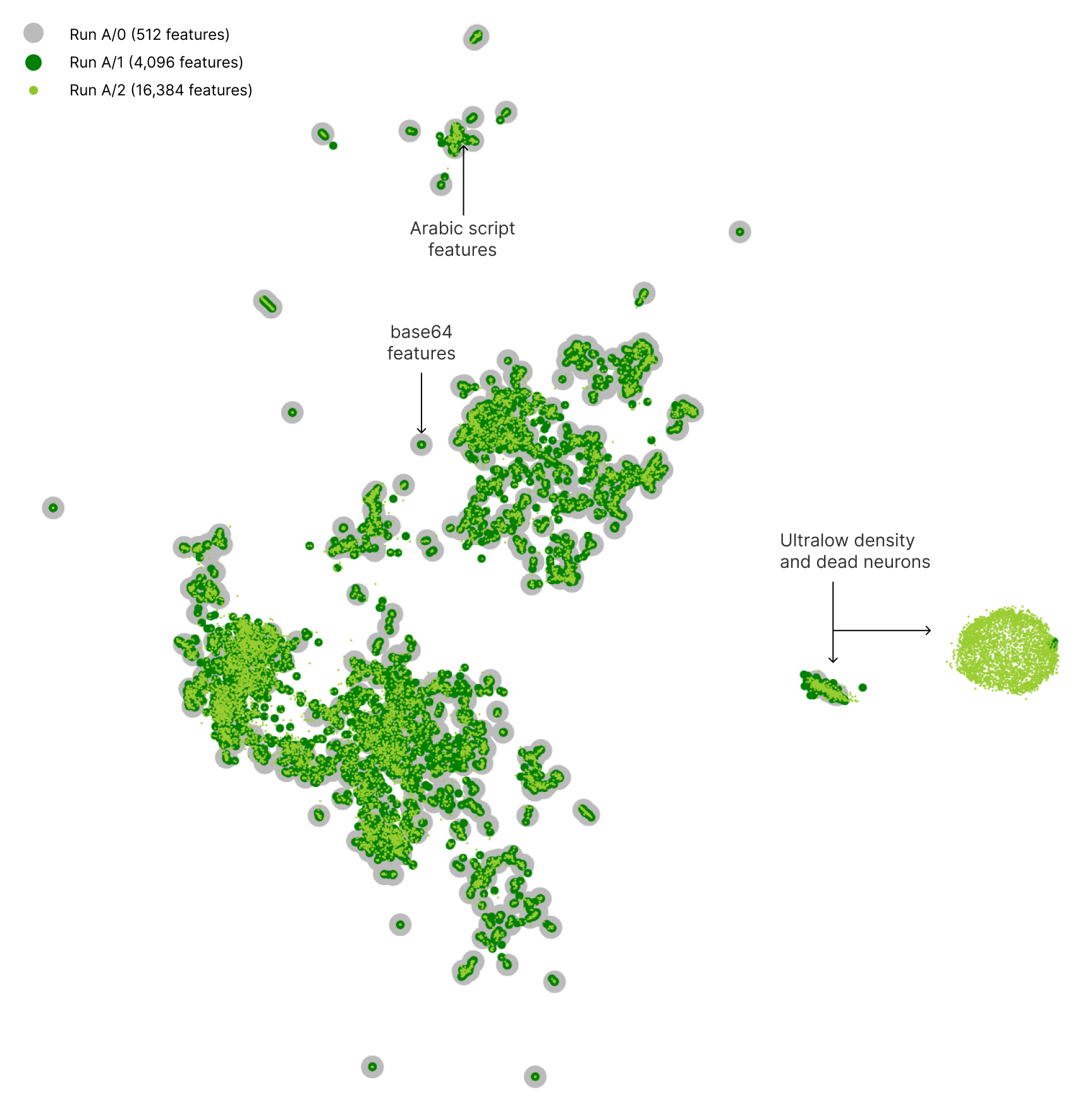
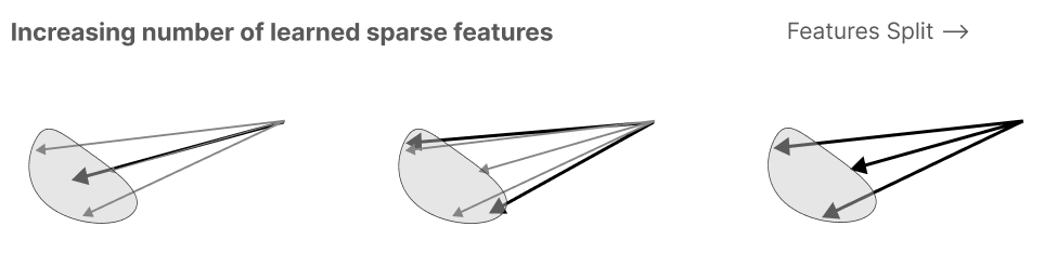
As dictionaries expand, coarse features subdivide into more specific related directions. Similarity in activations and output effects may explain why these directions cluster. The proposed picture of an ideal unlimited dictionary is conjectural; real features may also form continuous families.
Example: Mathematics and Physics Features
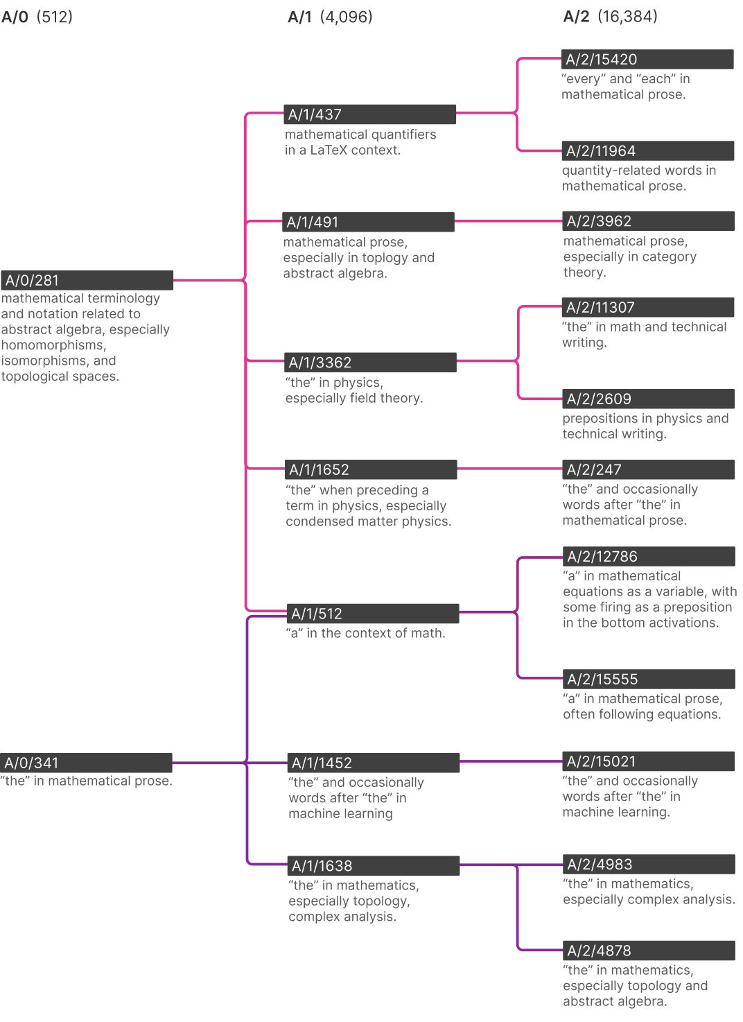
Technical-language features refine into distinctions among mathematics, machine learning, algebra, and physics, with corresponding differences in predicted nouns. The similarity graph can both split and merge, so refinement is not a simple tree.
Features which seemed like Bugs
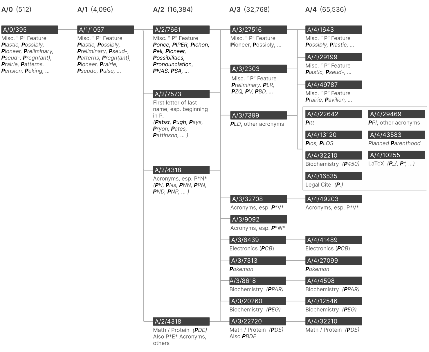
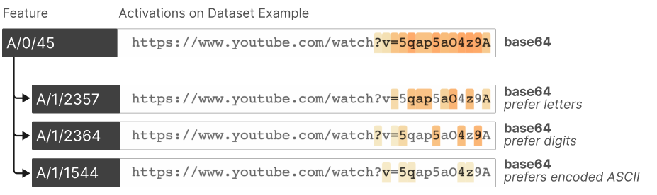
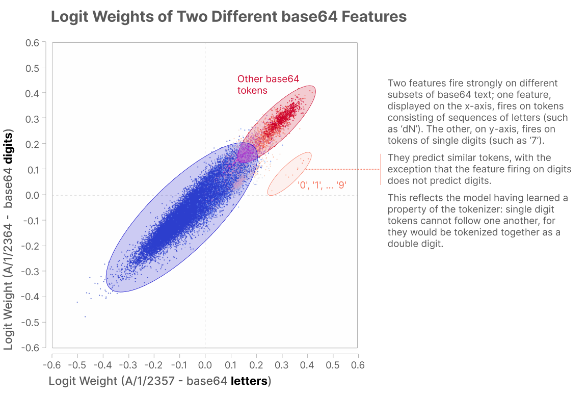
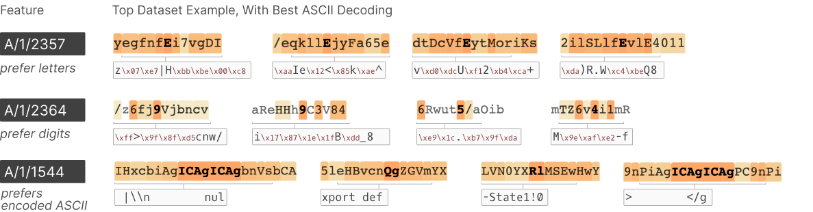
Apparently redundant single-token features can divide into context-specific variants at larger dictionary sizes. Three base64 features separate letters, digits, and strings encoding printable text; the digit feature exploits tokenizer constraints on which token may follow a single digit. Close inspection can therefore resolve some apparent decomposition errors.
Universality
Repeated features across models provide evidence of reproducibility. The strongest quantitative comparison uses two identically configured transformers with different seeds; comparisons to other architectures and papers are suggestive qualitative extensions.
Comparing features between two one-layer transformers
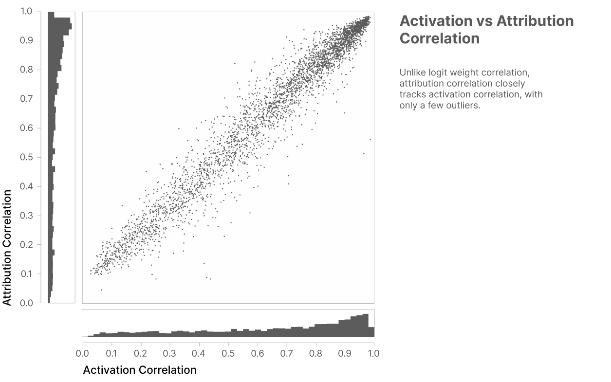
Matching features across models gives median activation correlation 0.72, versus 0.46 for matched neurons. Raw logit correlations can be much weaker because many small weights differ. Weighting feature activity by the next token’s logit contribution yields attribution similarities that better track activation similarity.
Comparing features with the literature
Comparable language, encoding, capitalization, and geographic features appear in earlier neuron and dictionary studies. These observations suggest broader recurrence, but person and emotion representations differ substantially across the systems compared.
"Finite State Automata"
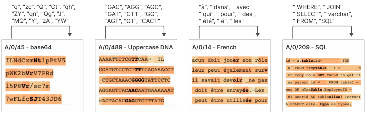
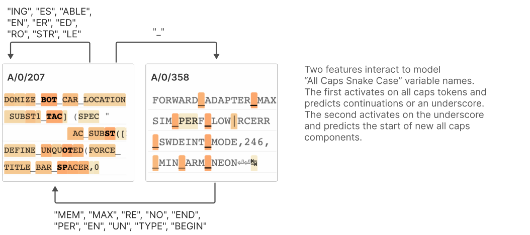
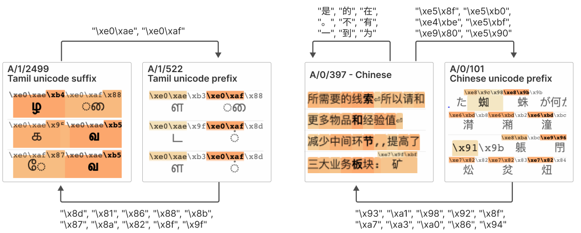
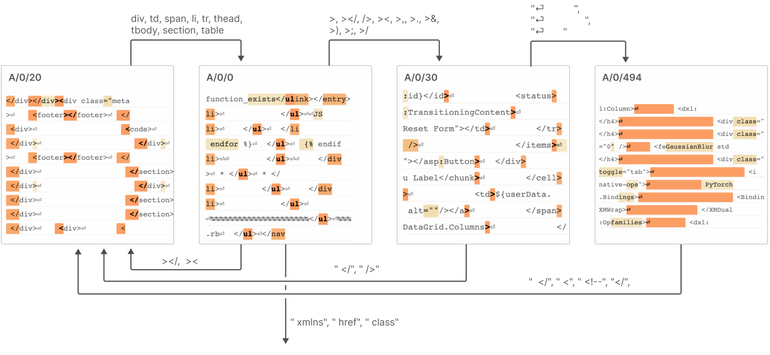
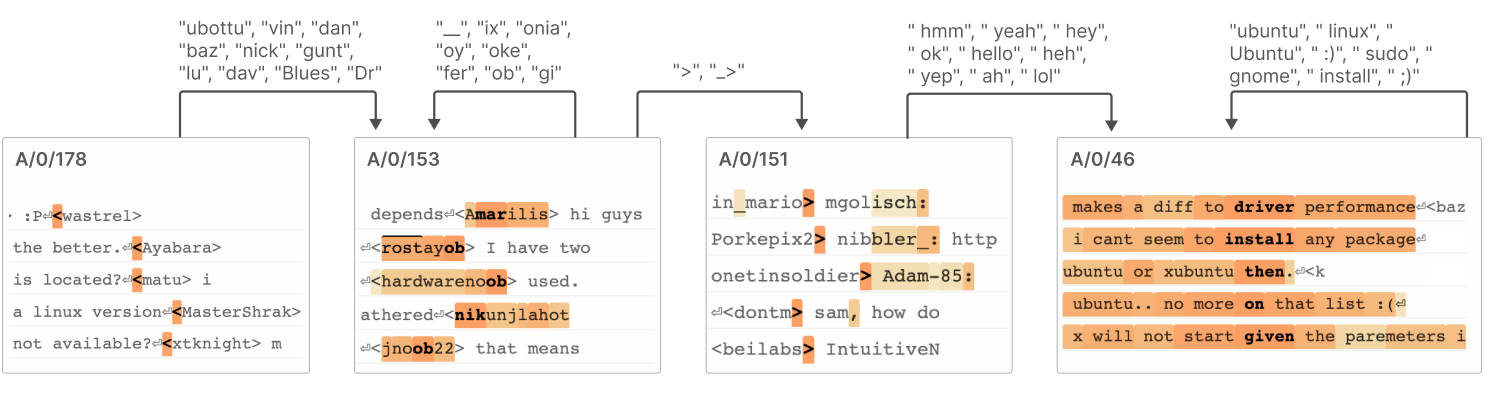
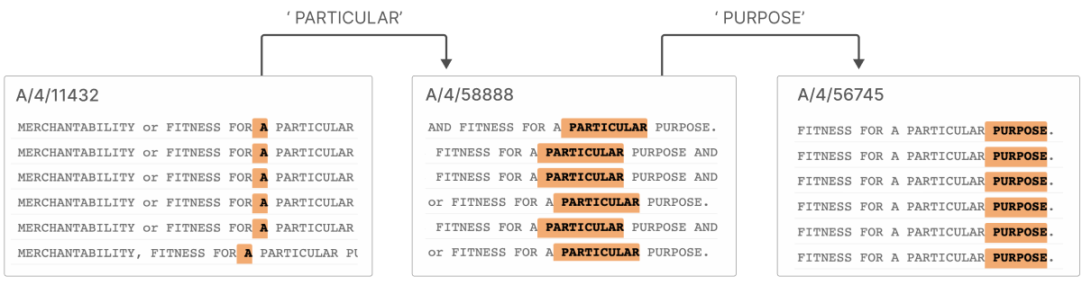
Features can promote tokens that activate themselves or other features on the next generation step. Examples cover base64, uppercase identifiers, split Unicode characters, HTML, chat transcripts, and a standard legal phrase. These are token-mediated, finite-state-like assemblies, rather than circuits whose components necessarily co-evolved as one explicit state machine.
Superposition
Subsequent toy-model studies examine when superposition forms, how dropout affects it, and how finite datasets can be memorized in shared dimensions. Sparse probes and alternative interpretations of learned game representations provide complementary evidence for linear features.
Disentanglement and Architectural Approaches
Disentanglement methods usually seek a manageable set of independent latent factors, whereas overcomplete dictionary learning permits more factors than dimensions. Architectural sparsity and SoLU can improve some neurons while leaving or worsening other mixtures; success depends on the task and loss.
Dictionary Learning and Features
Earlier work applies sparse coding to embeddings and transformer activations. Parallel reports by Sharkey, Cunningham, Smith, and Huben develop sparse autoencoders and automated evaluation with closely related findings. The paper explicitly credits that independent line of investigation.
Discussion
Crosscoders open new comparisons while raising questions about the relation between compact explanations and the model’s actual computation.
Theories of Superposition
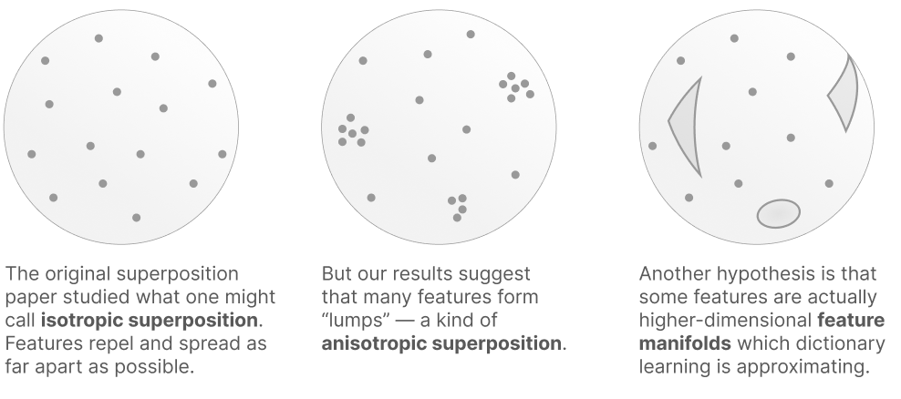
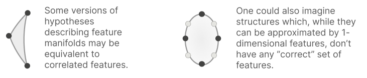
The findings challenge a purely uniform picture of repelling feature directions: related features cluster and may share output actions. Correlated groups or higher-dimensional manifolds could explain this organization. Under such possibilities, a single correct feature count may be ill-defined.
Are "Token in Context" Features Real?
Token-in-context features might reflect the transformer’s actual local code, an autoencoder preference for sparse combinations, or both. In a one-layer model, representing a conjunction separately can sharpen output predictions beyond simply adding token and context effects.
Future Work
Open problems include compute-efficient scaling, reliable feature-quality metrics, better sparse coding algorithms, attention representations, and explanations of interactions across many features. A successful decomposition alone would still leave the challenge of understanding the full model at larger scales.
Comments & Replications
The report includes an external replication and tutorial, which supplies an independent check and additional observations about dictionary behavior.
Replication & Tutorial
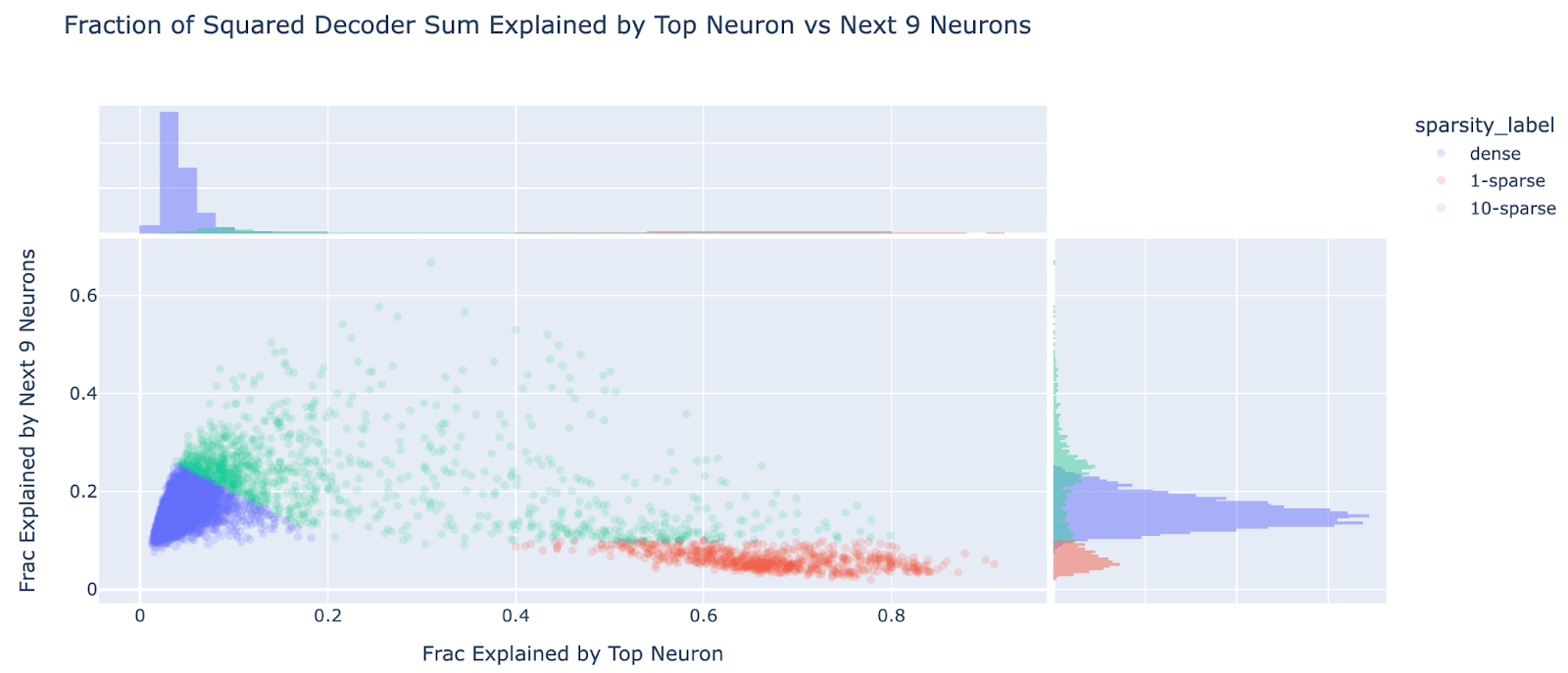
Neel Nanda replicates interpretable features in an open one-layer GELU model. Only 4% of decoder directions align well with one neuron, while 92% are dense. An ultrarare cluster shares a hard-to-interpret encoder direction, and median encoder–decoder cosine similarity is about 0.5, supporting untied weights.
Author Contributions Statement
The contribution statement describes the research, engineering, analysis, writing, and project support behind the report.
Infrastructure, Tooling, and Core Algorithmic Work
Bricken and Templeton develop the sparse-autoencoder procedure and scale its training, with contributions across infrastructure, metrics, ablations, and visualization. The named contributions distinguish algorithm development from the tooling needed to inspect billions of activations.
Analysis
The analysis combines feature case studies, a human scoring rubric, automated interpretation, splitting graphs, and cross-model comparisons. Different contributors build the associated ablation, sampling, and visualization tools.
Paper Production
Olah, Batson, and Jermyn lead drafting and revision; Templeton and Bricken write the training appendix. The figures combine analysis and illustration work from several authors.
Development of Intuition & Negative Results
Toy and small-image experiments inform the algorithms and reveal failed quality metrics. Chen’s sparse-architecture experiments and counterexample show that near-isolated neuron activations can still be polysemantic.
Other
Additional contributors support infrastructure, feature labeling, operations, and research management. Henighan leads the dictionary-learning project after its early phase under Hume.
Acknowledgments
The authors acknowledge external researchers and colleagues for technical feedback, feature exploration, and engineering support.
Citation Information
The publication is the 2023 Transformer Circuits report by Bricken and colleagues. The original citation record is retained with the source.
Bricken, et al., "Towards Monosemanticity: Decomposing Language Models With Dictionary Learning", Transformer Circuits Thread, 2023.
    @article{bricken2023monosemanticity,
       title={Towards Monosemanticity: Decomposing Language Models With Dictionary Learning},
       author={Bricken, Trenton and Templeton, Adly and Batson, Joshua and Chen, Brian and Jermyn, Adam and Conerly, Tom and Turner, Nick and Anil, Cem and Denison, Carson and Askell, Amanda and Lasenby, Robert and Wu, Yifan and Kravec, Shauna and Schiefer, Nicholas and Maxwell, Tim and Joseph, Nicholas and Hatfield-Dodds, Zac and Tamkin, Alex and Nguyen, Karina and McLean, Brayden and Burke, Josiah E and Hume, Tristan and Carter, Shan and Henighan, Tom and Olah, Christopher},
       year={2023},
       journal={Transformer Circuits Thread},
       note={https://transformer-circuits.pub/2023/monosemantic-features/index.html}
    }
Feature Proxies
Feature proxies compare a string’s estimated probability under a hypothesized context with its background probability. Maximizing over prefixes lets preceding tokens contribute evidence for the context.
Estimating the background probability
The background probability is approximated by multiplying empirical unigram token probabilities, which ignores dependencies between tokens.
Estimating base64 and character probabilities
Base64 and DNA proxies multiply uniform probabilities over their allowed character sets and assign a tiny probability to other characters. These deliberately simple models can reject valid formatting or conflate related encodings.
Estimating Arabic and script probabilities
Script proxies use Unicode blocks and Bayes’ rule. Shared punctuation is treated as outside the script; incomplete token fragments receive empirical script-use estimates. These conventions explain some apparent feature–proxy disagreements.
Feature Ablations
Ablation subtracts a feature’s activation times its decoder direction from the actual MLP activation at every token, then completes the forward pass. The resulting next-token likelihood changes test a feature’s causal contribution while retaining the rest of the original activation.
Feature Interpretability Rubric
The rubric combines confidence, activation consistency, output-weight consistency, separation of inconsistent output effects, and specificity. The published item ranges are retained in the source; this composite judgment is not a calibrated probability that an interpretation is correct.
Feature Density Histograms
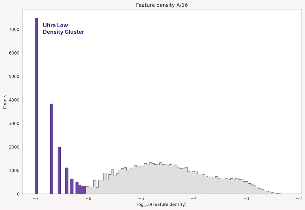
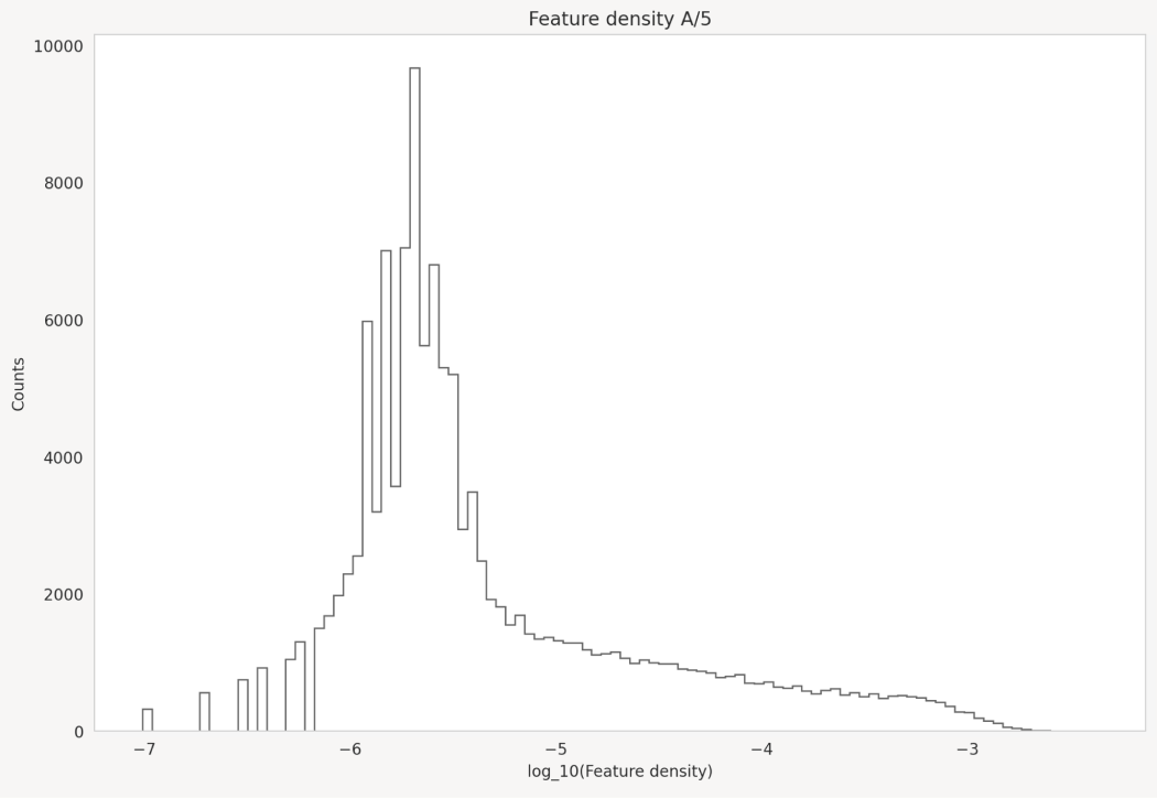
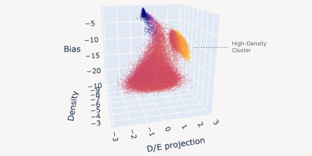
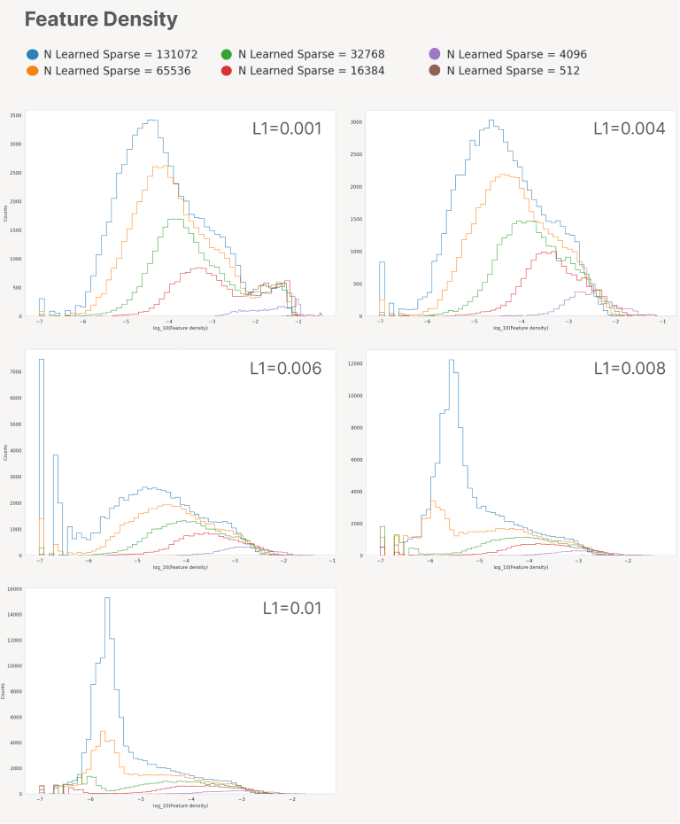
Density is the fraction of tokens with nonzero feature activity. Many runs contain an ultralow-density cluster that is rarely interpretable and appears to be a training artifact. Larger dictionaries continue to find additional rare features, so the experiments do not exhaust the model’s possible features.
Transformer Training and Preprocessing
Each transformer trains with Adam on 100 billion Pile tokens, using a 128-dimensional residual stream and 512-dimensional ReLU MLP. The public dataset supports reproducibility while also shaping which features appear.
Advice for Training Sparse Autoencoders: Autoencoder Dataset and Basic Training
The activation dataset samples 250 tokens from each of 40 million contexts. One million updates at batch size 8,192 use slightly over eight billion vectors without replacement. Mixing contexts and avoiding repeated examples improve the authors’ observed training behavior.
Advice for Training Sparse Autoencoders: Autoencoder Architecture
The encoder and decoder have independent weights; decoder columns are unit length. The objective combines reconstruction error and an L1 feature penalty. Implementation modifications are motivated by toy experiments and practical comparisons, rather than a complete controlled ablation of every interacting choice.
Equation
Pre-Encoder Bias
The same learned decoder bias is subtracted before encoding and added after decoding, initialized from the data’s geometric median. This recentering is important in the authors’ biased toy problems.
Decoder Weights Not Tied
Encoder directions detect features while avoiding interference; decoder directions reconstruct their contributions. Their empirical differences, including among nearby base64 features, motivate keeping the matrices untied.
Neuron Resampling
At steps 25,000, 50,000, 75,000, and 100,000, units inactive for 12,500 steps are reseeded from examples sampled proportional to squared reconstruction loss. Decoder vectors become unit length; encoder norms are set to 20% of the live-unit average, biases zeroed, and optimizer state reset. Resampling improves utilization but can cause loss spikes or divergence if too frequent.
Learning Rate Sweep
Lower learning rates, given enough updates, yield lower loss and more plausible features in the tested runs. Learning-rate annealing does not provide an additional observed improvement.
Interaction Between Adam and Decoder Normalization
Before applying Adam, the method removes decoder gradients parallel to each unit dictionary vector. This respects the fixed-norm constraint more directly than simply renormalizing afterward and produces a small loss improvement.
Advice for Training Sparse Autoencoders: Hyperparameter Selection
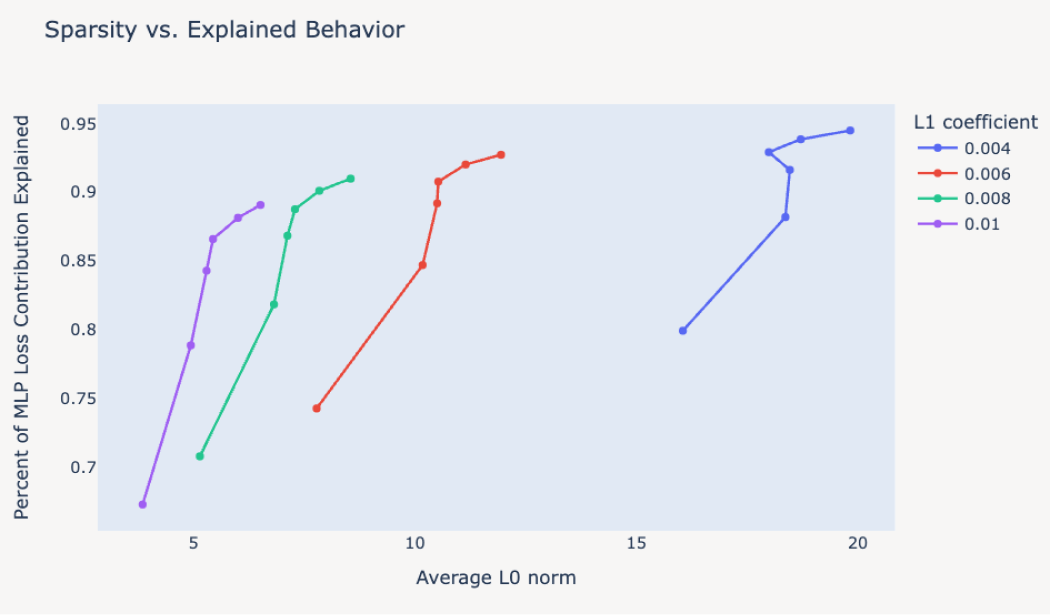
Hyperparameter selection combines loss, feature densities, active-feature count, and the transformer’s loss after reconstruction. Typical sparsity targets are below ten or twenty active features. Neither low reconstruction loss nor high loss recovery against zero ablation alone establishes interpretability; the baseline can overstate how much behavior is explained.
Activation Visualization
Activation illustrations use 100 million sampled tokens, with ten tokens per context and four neighboring tokens shown on either side. This sampling supports browsing but is distinct from the training and evaluation pools.
Feature UMAPs
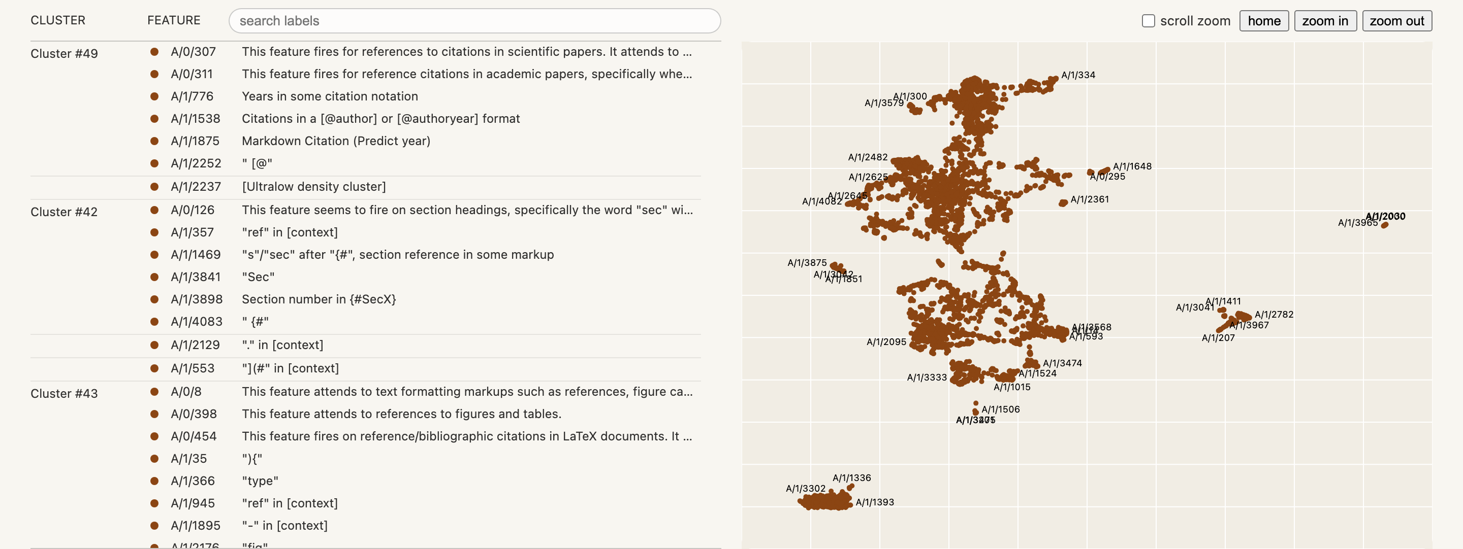
UMAP embeds decoder directions with cosine distance to show feature neighborhoods; HDBSCAN supplies clusters for one view. These visualizations organize high-dimensional geometry but do not prove a unique clustering or hierarchy.
Automated Interpretability
The additional evaluation details separate explanation generation, held-out prediction, randomized-model controls, and weighting choices.
Experimental Setup
Claude receives up to 49 explanation examples plus held-out demonstrations, then predicts activations for 60 different examples. A separate balanced test uses 50 held-out high-weight logits and 50 random logits. The appendix reports median logit accuracy 0.74 for features versus 0.53 for neurons, distinct from the main text’s mean comparison.
Randomized Transformer
Randomized-model dictionaries can score well on activation prediction because many features are trivial single-token detectors. Their output effects remain uninterpretable or near chance. This control shows why activation predictability alone is insufficient evidence of understanding a trained model.
Importance Scoring
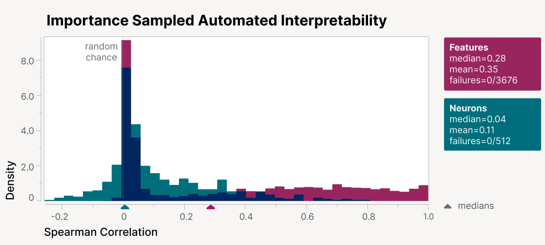
Importance weighting attempts to correct deliberately oversampled active intervals. Extremely sparse features place most weight on random examples where they are inactive, making false positives especially costly and sometimes favoring overly restrictive explanations. The weighted scores therefore answer a different question from interval-balanced evaluation.
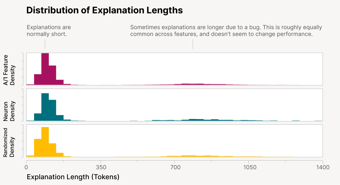
Explanation Lengths Caveat
Occasional missing answer tags leave longer explanations in the evaluation: 13% for features, 19% for neurons, and 15% for randomized-model features. Splitting results by explanation length does not substantially change the reported comparison, though automated interpretation remains an imperfect proxy.