Overview
The supplementary material derives the inner-box geometry, adapts inference to outer views, and supplies implementation details, runtime comparisons, and additional visual results.
At a glance
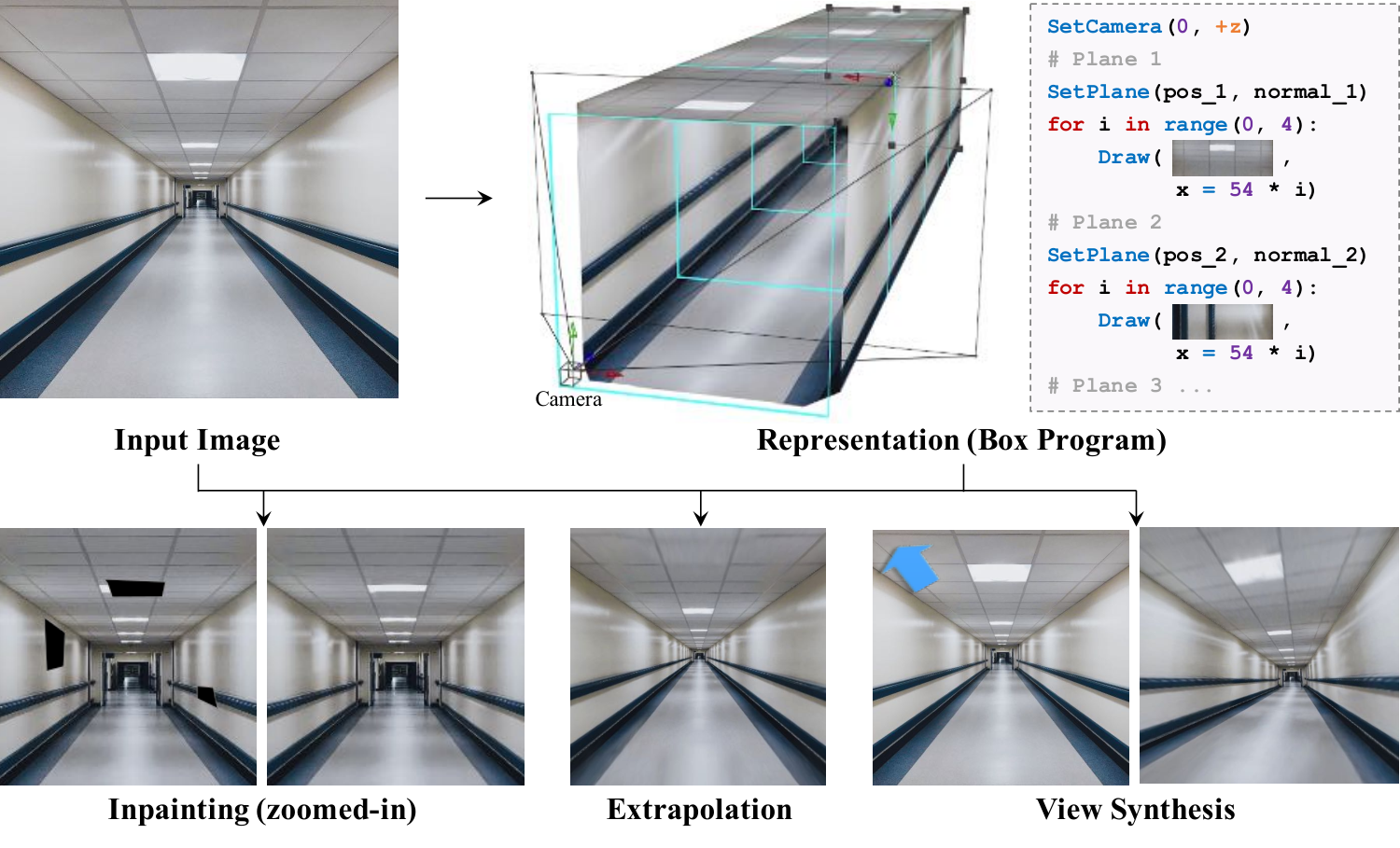
Box Program Induction infers an editable representation of repeated image patterns on several planar surfaces from one image. A box prior constrains the scene to an interior with four modeled planes or an exterior with two side walls. Learned vanishing-point and wireframe cues guide a search over plane partitions and repeating programs. The resulting representation supports perspective-aware inpainting, extrapolation, and view changes. Its geometric reconstruction depends on camera and scale assumptions rather than recovering absolute scene dimensions.
1 Introduction
A corridor or building contains both repeated patterns and perspective relationships among multiple surfaces. Programs fitted to a single plane miss this joint structure. BPI combines a restricted box geometry with learned visual proposals and an image-based regularity score. The chosen program partitions and rectifies surfaces, then describes their repeated elements with loops. This makes structured editing possible while restricting the method to scenes whose useful regions fit the planar, repeating assumptions.
2 Related Work
The related work connects visual program induction with patch-based and learned image editing.
Visual program induction.
Earlier procedural representations cover shapes, scenes, sketches, and image markup. Program-guided editing of natural images usually assumes one visible plane. BPI extends Perspective Plane Program Induction [21] to multiple surfaces by using box constraints to reduce the search. Its explicit geometric and repetition parameters are intended for editing, beyond merely reproducing an image.
Image manipulation.
Patch matching supplies local texture but can violate larger structures. Perspective-aware methods rectify surfaces, and learned inpainting supplies semantic priors. BPI instead uses the input image’s pixels together with inferred plane geometry and lattice regularity. Pretrained visual-cue networks still contribute external learned information.
3 Box Program Induction
Inference proposes a box-shaped plane partition, fits repeated programs to rectified planes, and chooses the best combined image agreement.
3.1 Domain-Specific Language
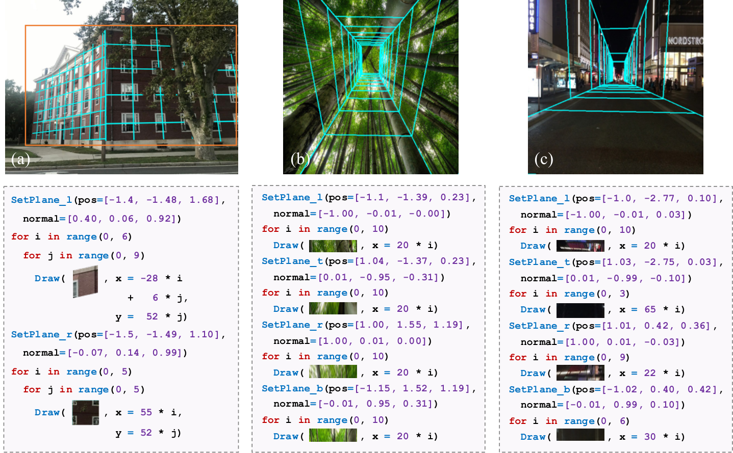
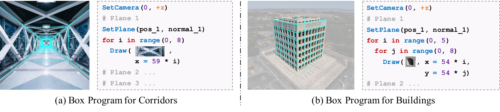
A box program specifies camera parameters and a program for each surface. Each plane has a normal and repeated Draw operations inside up to two nested For loops. The grammar represents lattice patterns rather than arbitrary scene semantics; Table 1 retains its precise syntax and Figure 2 illustrates interior and exterior programs.
| Program | CameraProgram; WorldProgram; | |
| CameraProgram | SetCamera(pos=Vec3, point_to=Vec3); | |
| WorldProgram | PlaneProgram; PlaneProgram; World Program; | |
| PlaneProgram | SetPlane(pos=Vec3, normal=Vec3) For1Stmt; | |
| For1Stmt | For ( in range(Integer, Integer) ){ DrawStmt; For2Stmt } | |
| For2Stmt | For ( in range(Integer, Integer) ){ DrawStmt } | |
| DrawStmt | Draw (=Expr, =Expr) | |
| Expr |
3.2 Box Program Fitness
Each candidate plane is rectified to remove perspective effects. A lattice program predicts centers of repeated elements; fitness compares image patches at neighboring repetitions. For lattice patterns, this can be evaluated by shifting the rectified image by one cell and measuring pixel differences. Scores sum across planes, so a candidate must explain both the partition and the visual repetition.
Equation 1
| (1) |
3.3 3D Box Priors and the Role of Visual Cues
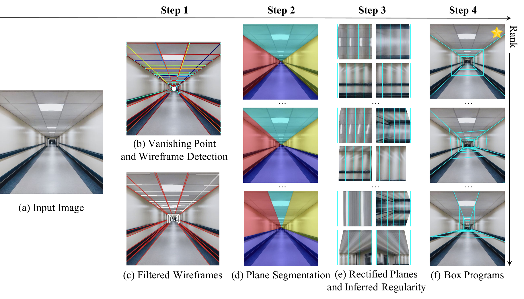
An interior models two walls, floor, and ceiling; the far plane is segmented but excluded from program modeling. An exterior models two side walls, leaving the roof unmodeled. These priors restrict the combinatorial search. The main procedure below concerns interiors; Appendix B handles exteriors.
Step 1: Visual cue detection.
NeurVPS [47] supplies the most confident vanishing point, and L-CNN [48] supplies line segments. Short segments and segments whose extended lines miss a small neighborhood of the vanishing point are removed. Remaining lines propose the four plane intersections.
Step 2: Plane segmentation.
Every combination of four surviving segments yields a candidate partition. Because predicted lines may not meet exactly, the procedure refits a common vanishing point by minimizing distances to their extended lines. Rays from that point through the segments partition the image into four regions.
Step 3: Plane rectification and regularity inference.
The camera is fixed at the origin with a 35 mm focal length, zero skew, and unit pixel aspect ratio. Plane geometry derived from the candidate rays enables rectification and a search over lattice programs. Appendix A additionally fixes a one-meter normalization to resolve scale ambiguity. Thus the reconstruction supplies a consistent geometry for editing under these assumptions, not a uniquely measured metric scene.
Step 4: Box program ranking.
The four plane fitness values are summed, and the highest-scoring candidate becomes the image’s box program. Regularity therefore helps select among noisy geometric proposals.
3.4 Program-Guided Image Manipulation
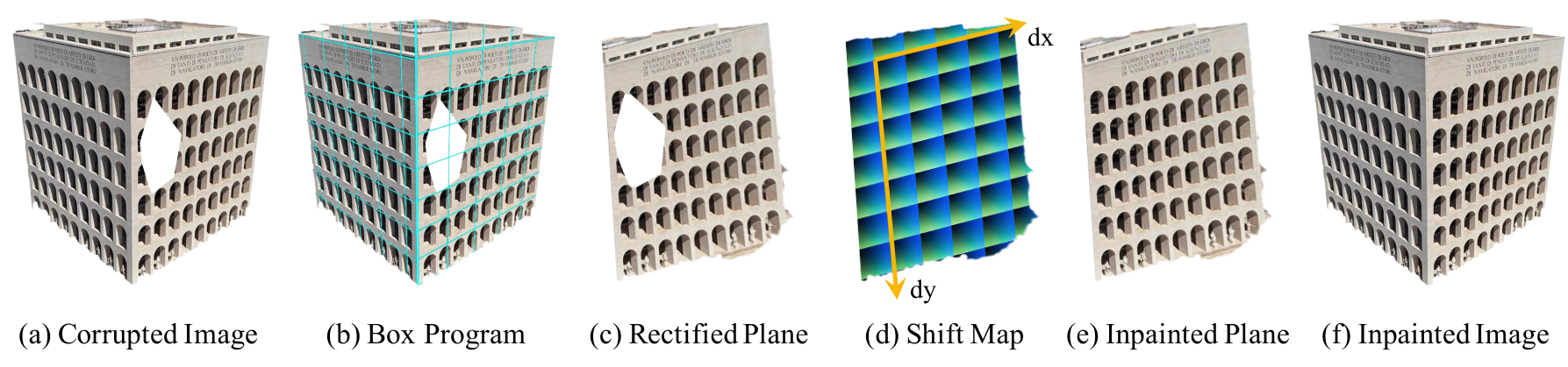
The editing stage augments PatchMatch [4] with a regularity term. After rectification, a shift map records each pixel’s location within a repeating lattice cell. Candidate patches are favored when they match both appearance and corresponding positions in the repeated pattern, including periodic wraparound. The same mechanism fills missing pixels or extends surfaces beyond the input image for extrapolation and camera changes.
Equation 2
| (2) |
4 Experiments
Experiments evaluate segmentation, inpainting, extrapolation, and novel-view synthesis on small, specifically collected sets of box-like scenes.
Dataset.
The datasets contain 44 corridor and 42 building images from web searches. Plane boundaries are manually annotated; corridor far planes and building foreground subjects also receive masks. These annotations and scene selection define a narrower setting than unrestricted natural images.
4.1 Plane Segmentation
Segmentation is obtained by the program search rather than by directly predicting supervised plane labels. The intended advantage is that a good partition makes the repeated visual elements easier to explain.
Baselines.
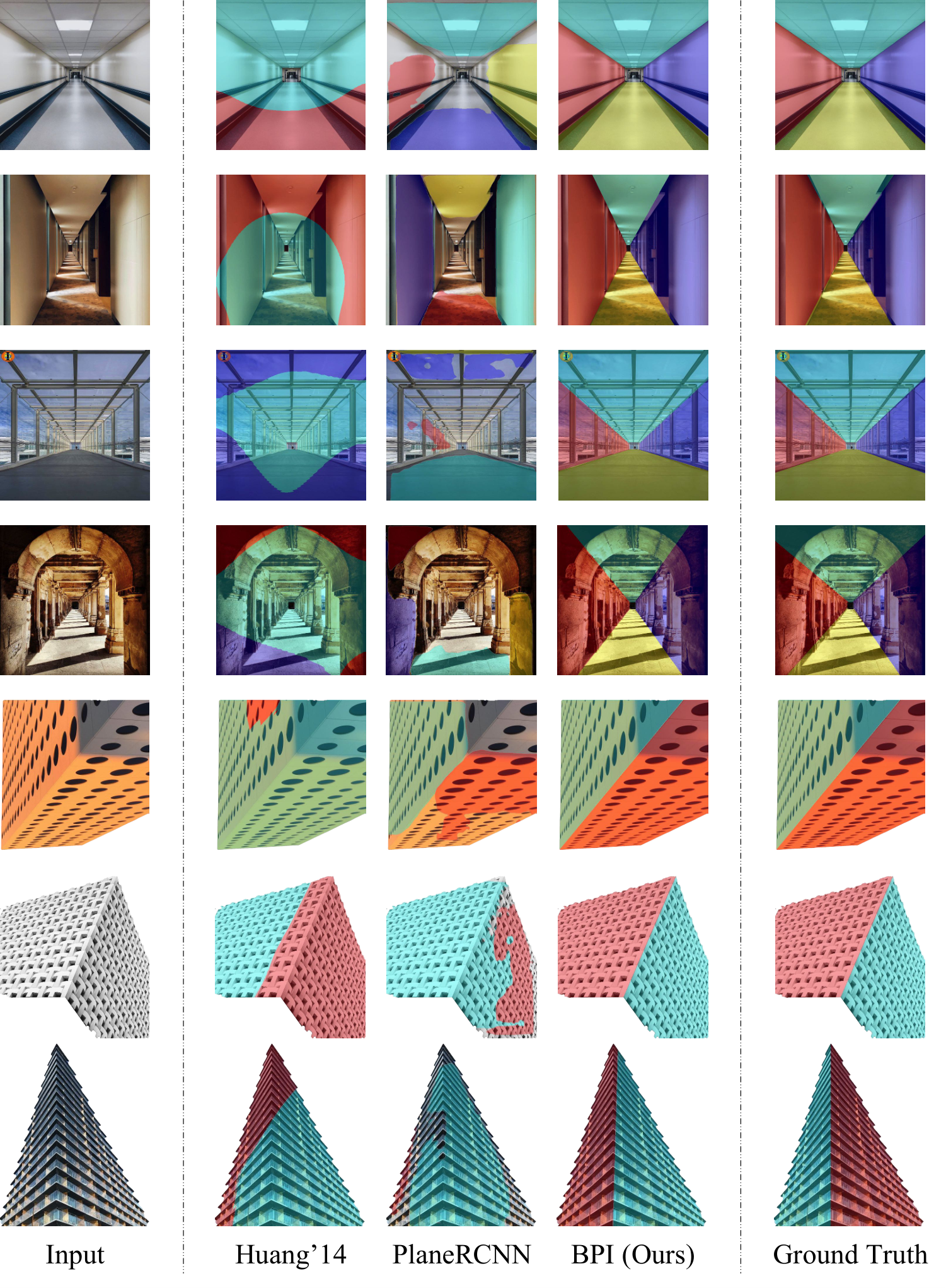
The comparisons use Huang et al.’s line- and vanishing-point-based method and PlaneRCNN, trained on ScanNet. Their different learned data and geometric assumptions should be considered when interpreting the small custom datasets.
| Method | CrdO | CrdC | BldO | BldC |
| Huang et al. [16] | 0.30 | 0.30 | 0.73 | 0.69 |
| PlaneRCNN | 0.52 | 0.52 | 0.63 | 0.63 |
| BPI (Ours) | 0.84 | 0.84 | 0.86 | 0.86 |
Metrics.
Predicted masks are matched to annotations by intersection over union, and their mean overlap is reported. Corridor far-plane pixels are excluded. Both original and randomly corrupted images are evaluated because segmentation must also work as an input to inpainting.

Results.
BPI reaches mean intersection over union of 0.84 on both original and corrupted corridors and 0.86 on both building conditions. PlaneRCNN obtains 0.52 and 0.63, respectively; Huang et al. obtains 0.30 on corridors and 0.73/0.69 on buildings. The examples show improved partitions around complex repeated structures within these datasets.
4.2 Image Inpainting
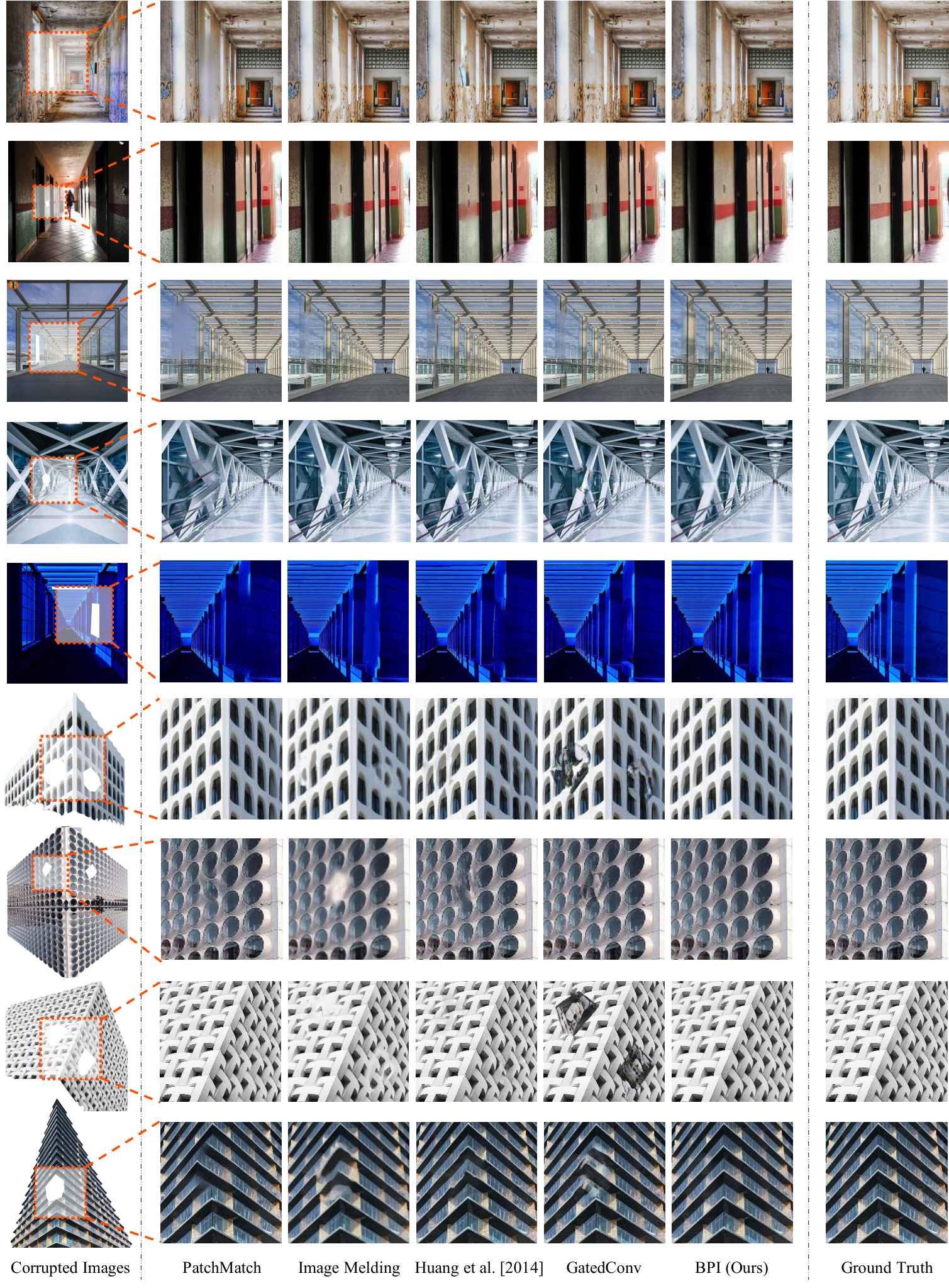
Random masks remove image regions, and the inferred programs guide their reconstruction. This tests whether the structure inferred from undamaged pixels improves completion.
Metrics.
Evaluation reports pixel L1 error, peak signal-to-noise ratio, structural similarity, and learned perceptual distance. The middle two are computed on luma; L1 and perceptual distance use RGB. The metrics assess different properties and do not have identical winners.
Baselines.
Baselines include GatedConv, ordinary PatchMatch, Image Melding with additional patch transformations, and Huang et al.’s perspective-corrected patch matching. The comparison isolates the value of structured editing only imperfectly because each full pipeline differs.
| Corridors | Buildings | |||||||
| Method | Mean | PSNR | SSIM | LPIPS | Mean | PSNR | SSIM | LPIPS |
| PatchMatch | 53.12 | 31.55 | 0.9872 | 0.0215 | 34.88 | 32.99 | 0.9896 | 0.0072 |
| Image Melding | 58.50 | 30.54 | 0.9880 | 0.0174 | 49.10 | 30.42 | 0.9890 | 0.0134 |
| Huang et al. [16] | 51.88 | 31.41 | 0.9869 | 0.0177 | 26.10 | 34.87 | 0.9917 | 0.0049 |
| GatedConv | 44.98 | 32.32 | 0.9883 | 0.0153 | 55.31 | 29.54 | 0.9866 | 0.0112 |
| BPI (Ours) | 38.45 | 34.21 | 0.9892 | 0.0170 | 26.43 | 34.86 | 0.9913 | 0.0054 |
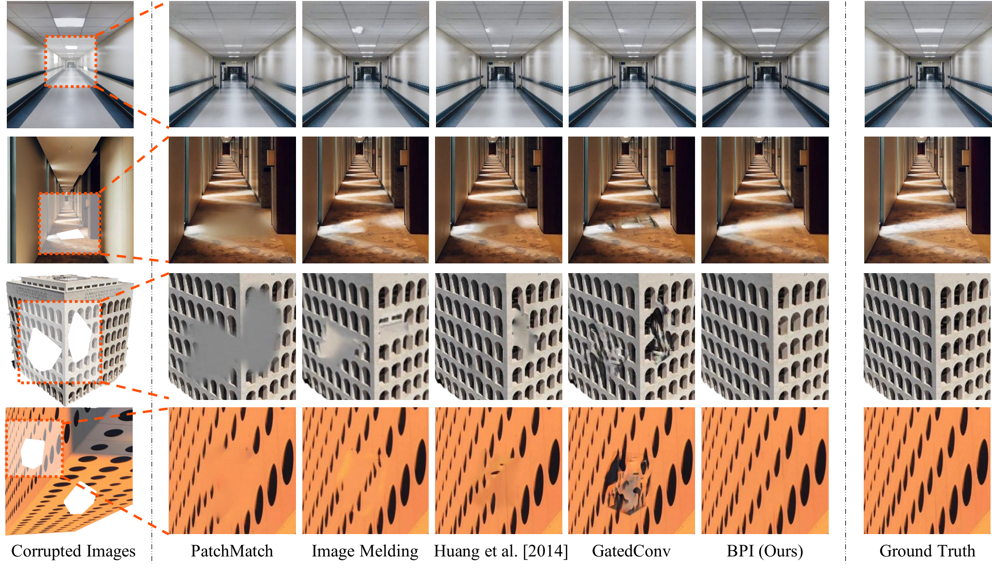
Results.
On corridors, BPI obtains L1 error 38.45, PSNR 34.21, and SSIM 0.9892, improving these point estimates over the listed baselines. GatedConv has the better LPIPS value, 0.0153 versus 0.0170. On buildings, BPI is close to Huang et al., whose point estimates are slightly better on all four measures. Bold entries denote the paper’s pairwise mixed-model tests, not proof that methods are equivalent. The qualitative examples highlight preservation of ceiling lights and other regular patterns.
Image extrapolation.
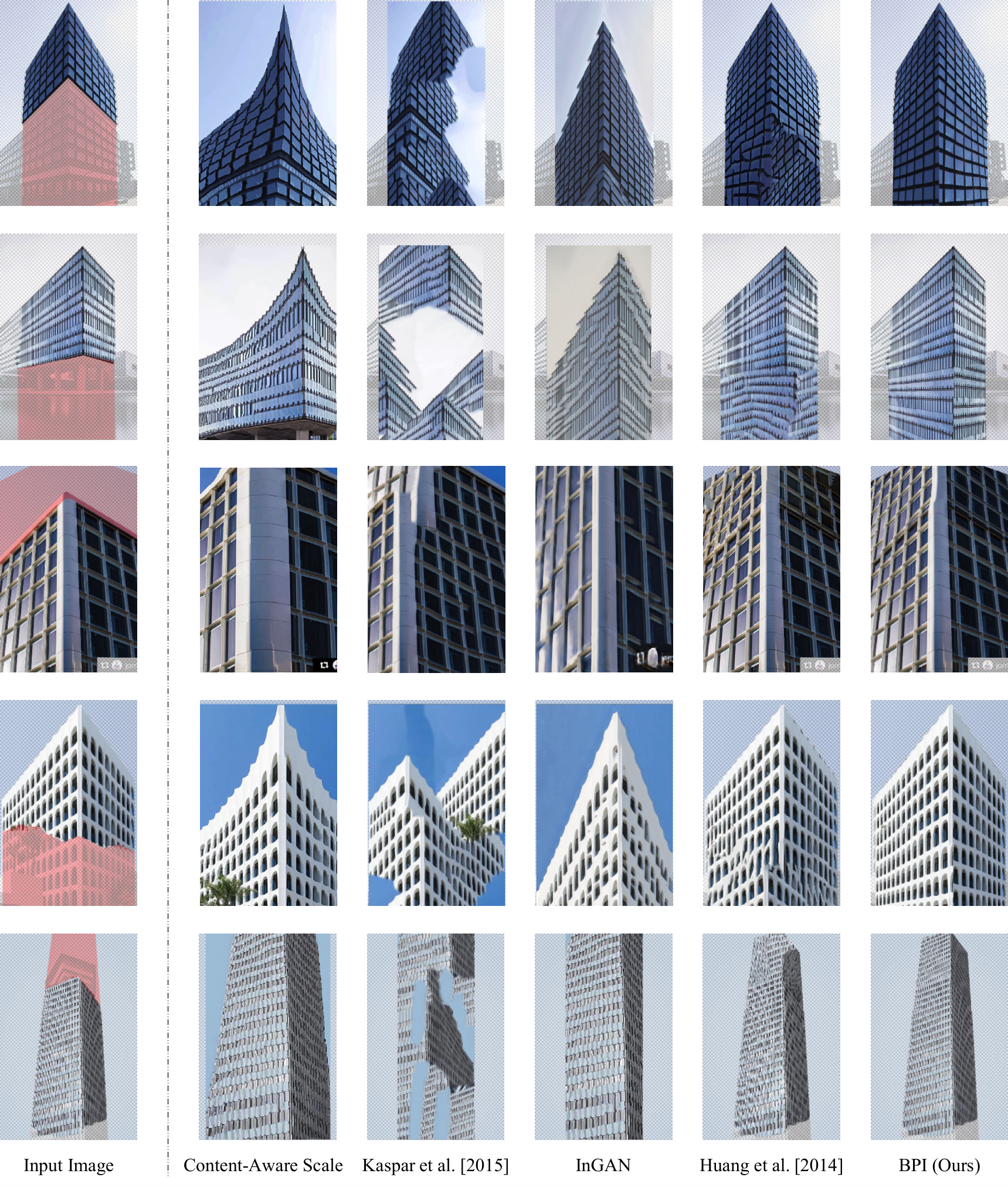
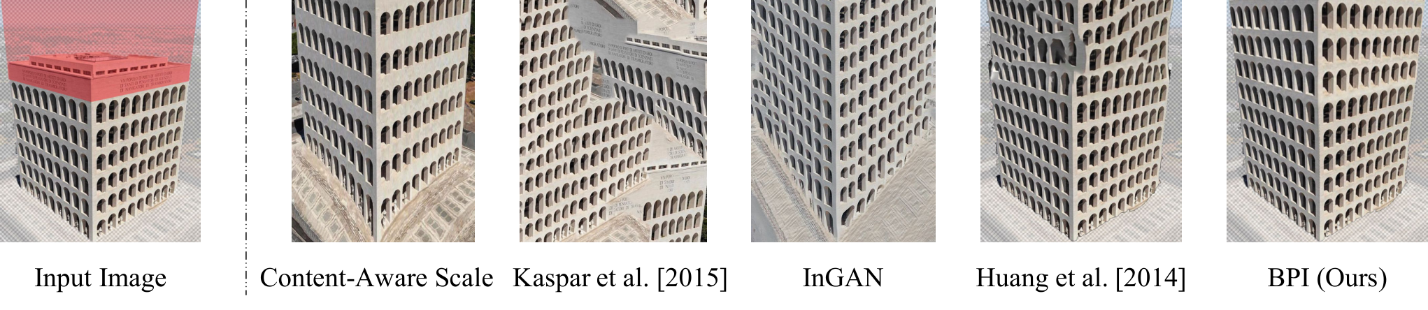
Extrapolation receives a foreground building mask and target fill region, then extends regular surfaces into that region. Compared methods include Photoshop content-aware scaling, texture synthesis, InGAN, and Huang et al. Fifteen people rank outputs for twelve images: 61% of 180 responses favor BPI, versus 16%, 2%, 16%, and 5% for those alternatives. This measures preference on selected outputs, not recovery of unseen real building structure.
4.3 View Synthesis
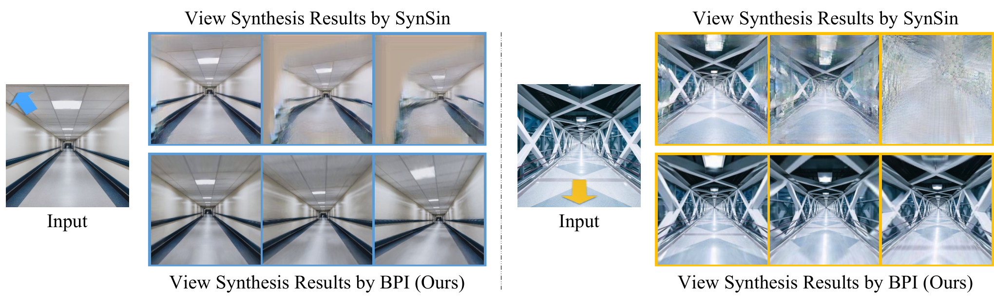
Three five-frame trajectories move forward, backward, or backward with a pan and tilt through corridor scenes. Backward motion exposes unobserved image regions, which program-guided matching fills by extending the inferred repetition. The output is a plausible structured synthesis rather than observed novel-view ground truth.
Results.
Compared with SynSin [38], BPI receives 100%, 94%, and 99.5% preference for the three trajectories. The study uses twenty images and ten raters, producing 600 responses. These strong preferences support perceptual quality for this regular corridor setting, while leaving metric geometric accuracy and general-scene performance untested.
4.4 Failure Case
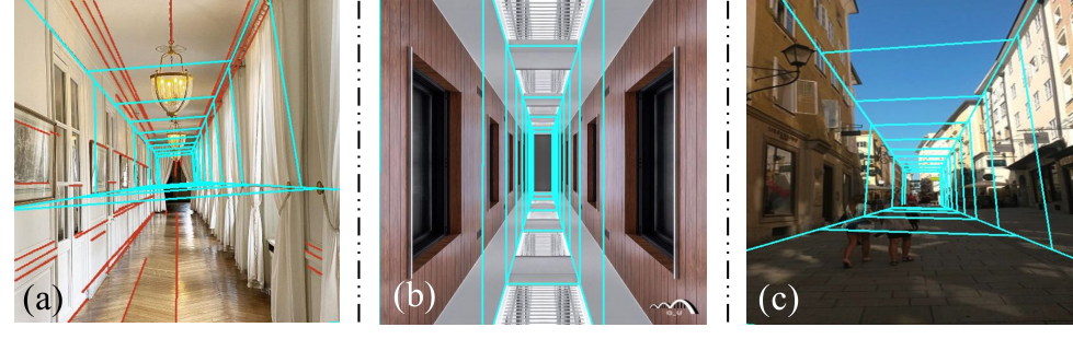
Failures arise from missing or incorrect line/vanishing-point cues, solid-color surfaces that provide ambiguous partitions, and irregular surfaces that violate the box prior. User-specified wireframes can help. The resulting interaction is a possible repair, not evidence that inference succeeds automatically on those cases.
5 Conclusion
Joint geometry and repetition inference makes several image edits possible from one constrained representation. The principal limitation is the assumption that relevant regions are planar and regularly structured. Incorporating irregular regions remains a proposed extension.
Broader Impact
The intended beneficiaries are people making content-aware and perspective-aware image edits. Reusing source pixels reduces dependence on external image content, although the cue detectors remain pretrained. The authors also identify fabricated imagery and image-forensics misuse as possible consequences.
Acknowledgements
The acknowledgments identify support from the Center for Brains, Minds and Machines, NSF, ONR, and IBM Research, and note Jiajun Wu’s visiting appointment at Google Research.
Appendix A Plane Reconstruction from Segmentation in Inner Views
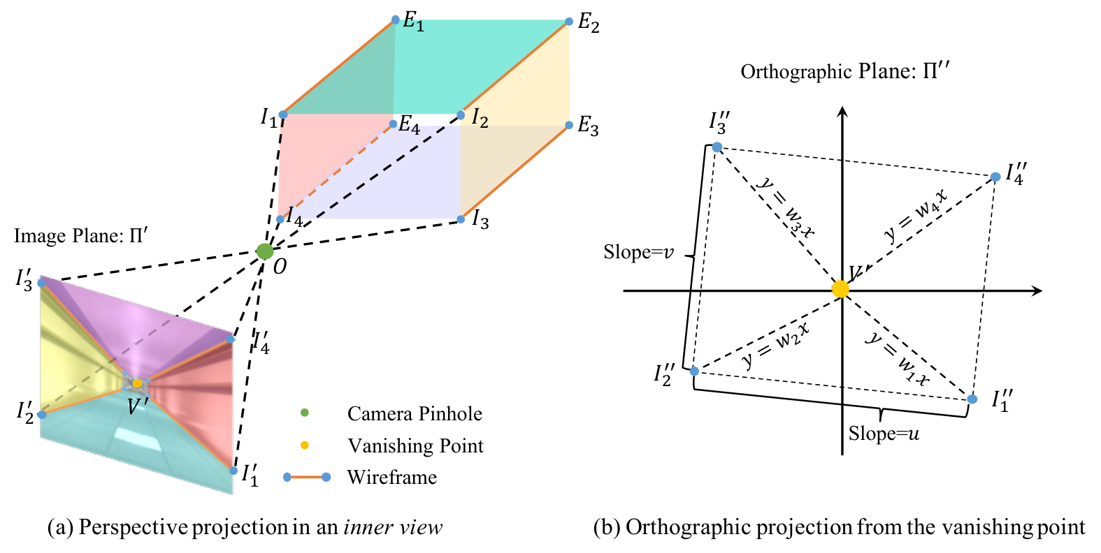
The derivation assumes a distortion-free pinhole camera. Four image rays through the vanishing point represent intersections among the interior planes. Projecting along the vanishing direction produces a cross-section whose four corners must form a rectangle: opposite edges are parallel and adjacent edges perpendicular. The retained equation system solves the relative corner positions and hence the surface normals.
Camera focal length, aspect ratio, distance, and box size are not jointly identifiable from this image. The derivation fixes focal length at 35 mm and aspect ratio at one, then manually fixes one projected distance to one meter. This final normalization removes the remaining scale ambiguity. The authors state that these choices do not alter the rectification and downstream inpainting results; they should not be read as recovered physical dimensions.
Equation
Appendix B Box Program Induction for Outer Views of Boxes
For exterior views, only two side planes are considered. The process again proposes partitions, infers each surface’s repetition, and ranks the combined program, but it does not use a vanishing-point detector.
Step 1: Visual cue detection.
L-CNN detects candidate wall-intersection line segments. Short segments are filtered; the vanishing-point proximity filter used for interiors is omitted.
Step 2: Plane segmentation.
Each surviving segment is extended to a line that divides the image into two candidate plane regions.
Step 3: Plane rectification and regularity inference.
Two-plane segmentation alone does not determine full geometry. The P3I algorithm jointly searches for surface normal and repeating program separately on each region, using image regularity to constrain perspective.
Step 4: Box program ranking.
The two plane scores are summed, and the highest-scoring partition/program pair is retained.
Appendix C Implementation Details
The minimum line length is 10% of the shorter image dimension; the interior vanishing-point filter radius is 1%. Rectified planes are resized to 200 × 200 pixels for inference. At least three repetitions per plane are assumed, a material constraint on suitable inputs.
Appendix D Additional Results
Additional results retain runtime tables and complete visual comparisons for programs, segmentation, completion, and extrapolation.
Time complexity.
A corridor image averages 1,506 line combinations and 46 programs evaluated per plane. The box prior gives a reported 23-fold search speedup over removing that prior; it does not make BPI the fastest listed system. Segmentation takes 43.50 s for corridors and 171.20 s for buildings, versus PlaneRCNN’s 0.14 and 0.76 s. Inpainting takes 20.1 and 41.4 s, versus GatedConv’s 1.9 and 4.9 s. Huang et al. and Image Melding run on a different CPU machine from the remaining methods, so cross-method timing also reflects hardware differences.
Qualitative results.
Figures 11–14 retain the supplementary program examples and all segmentation, inpainting, and extrapolation comparisons. User-selected regions allow selected less regular examples, including a curved wall and bamboo scene. These illustrations show possible extensions with interaction; they do not constitute a separate broad benchmark beyond the two box datasets.
| Huang et al. [16] | PlaneRCNN [23] | BPI (Ours) | |
| Corridor Boxes | 1.91s | 0.14s | 43.50s |
| Building Boxes | 6.83s | 0.76s | 171.20s |
| PatchMatch [4] | Image Melding [7] | Huang et al. [16] | Gated Conv [44] | BPI (Ours) | |
| Corridor Boxes | 61.6s | 1275.1s | 18.9s | 1.9s | 20.1s |
| Building Boxes | 122.1s | 808.3s | 64.4s | 4.9s | 41.4s |