Products of experts combine task-space preferences into a normalized distribution over robot configurations. Learning the factors jointly helps separate intended goals from kinematic restrictions and competing tasks. Variational mixtures approximate the otherwise difficult normalization.
A null-space extension recovers secondary objectives hidden by higher-priority tasks. Evidence includes planar simulations, Panda configuration experiments, and physical tray serving. The framework uses structured task transformations and kinematics; it does not learn arbitrary robot skills directly from images.
1 Introduction
Learning each task-space model independently can confuse demonstrated variability with what a task allows. Joint normalization asks which complete configurations the combined model predicts, allowing constraints and dependencies to influence learning.
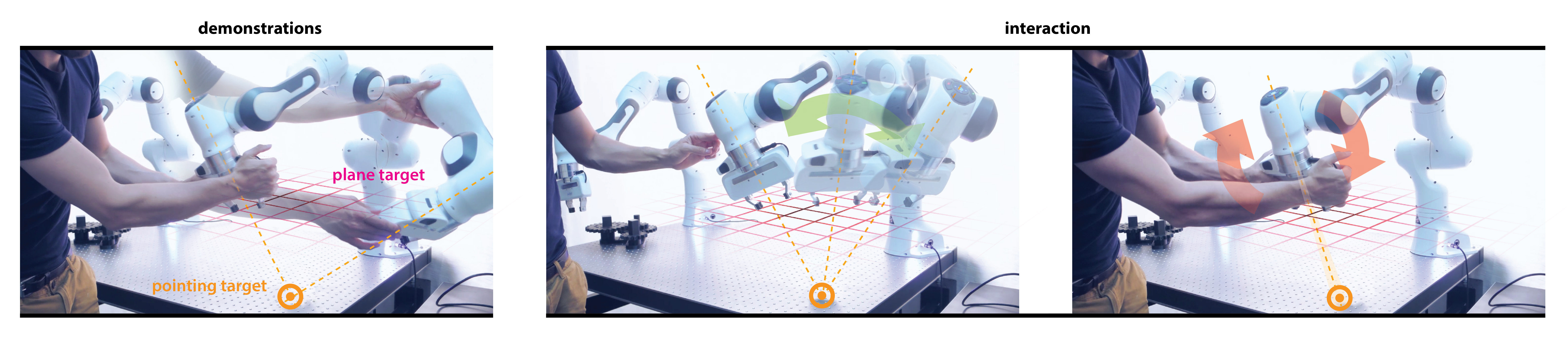
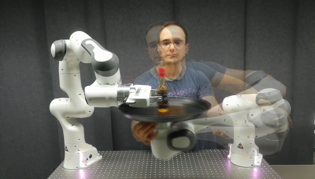
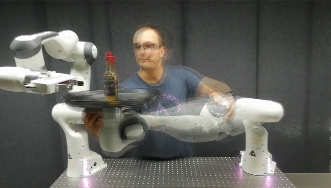
Figure 1: Product of experts can be used to set up virtual guides on robotic manipulators. A user demonstrates kinesthetically several configurations fulfilling the task objectives (left). In this example, the end-effector of the robot should stay close to a horizontal plane, while pointing to a desired target. The objectives are then inferred by the robot as target distributions under several transformations (task spaces). By exploiting the torque control capabilities of recent robots, the different objectives are tracked. Using an optimal control strategy, feedback gains can be computed according to the precision of the different objectives. As a resulting behavior, the robot is free to move along directions that are not constrained by the objectives (center), while preventing deviations from the objectives (right).
Organization of the article
The paper develops product-of-experts estimation, a null-space extension, a toolkit of robot transformations and distributions, two control strategies, and experiments testing their advantages.
Figure 2:
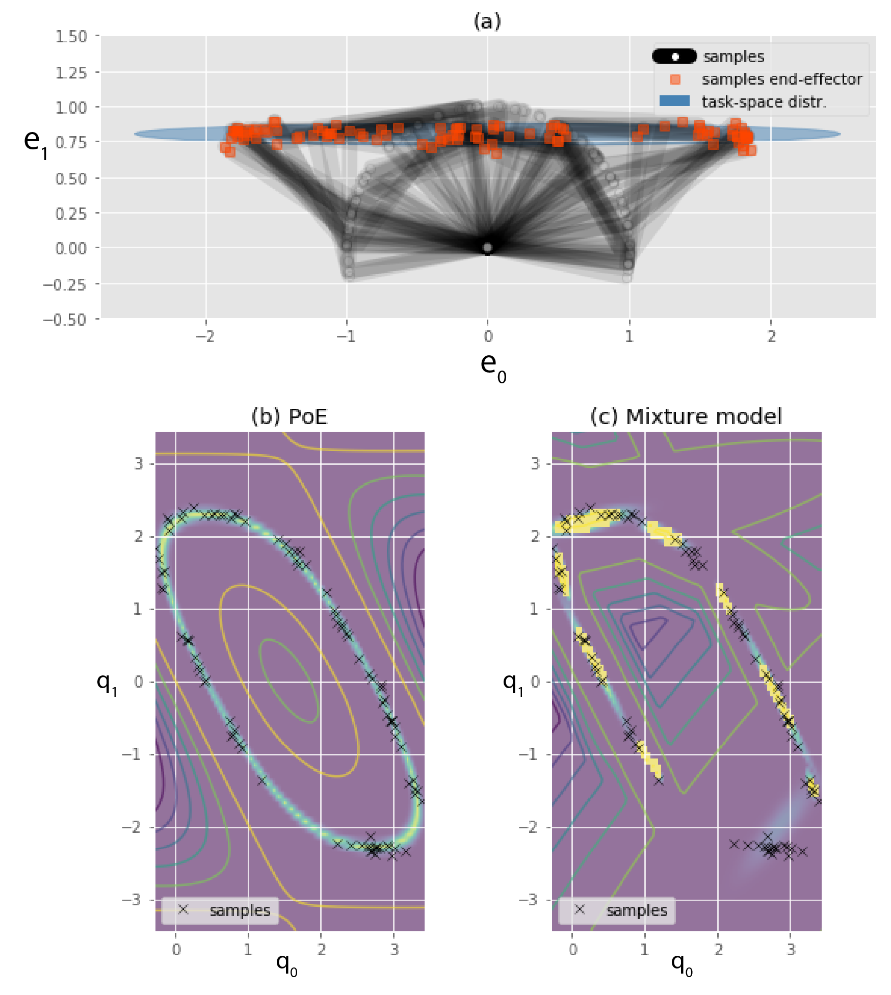
Product of experts can learn complex distributions of joint angles as a fusion of simple distributions within several task spaces.
(a) 30 samples of the configuration of a 2-DoF planar robot are displayed. The end-effector follows an elongated Gaussian distribution. The distribution in configuration space has a more complex shape, which it is difficult to represent. (b) With our approach, we learn configuration-space distributions as a product of simple densities in different task spaces. It is thus possible to represent this sharp distribution easily with few parameters. (c) A standard approach like a Gaussian mixture model, directly applied in configuration space, needs much more samples and parameters to represent this distribution. Following Occam’s razor principle, finding simpler explanations (fewer parameters of the model) to understand complex dataset leads to better generalization.
1.1 Related work
The related work connects density estimation, compositional probabilistic models, robot imitation, and inverse optimal control.
Estimating distributions
General density estimators can represent complex data but often need many examples. Robot kinematics supplies useful structure: a complicated joint-space distribution may correspond to a simple target in task space.
Product of experts
In a mixture, any component can explain an observation. In a product, all experts jointly constrain it. The main difficulty is estimating the product’s normalization and learning its parameters.
Distributions for learning in robotics
Earlier robot methods frequently fit independent distributions and combine them only during control. Joint fitting instead accounts for reachable configurations and task interactions. It can infer hidden target preferences from static configurations, without requiring demonstrated control commands. This extends earlier task-priority learning, which required known task references. [57]
Inverse optimal control
Negative expert log-likelihoods act like task costs. Learning them resembles inverse optimal control, with more explicit structure and smaller demonstration datasets than general neural cost learning. The experiments primarily concern static configuration distributions.
Equation 1
(1)
2 Product of Experts
Each expert scores a transformation of the joint configuration. Multiplying these scores and integrating over configurations defines one distribution. Simple experts can produce sharply constrained, multimodal joint-space distributions because robot kinematics is nonlinear.
Equations 2–3
(2)
(3)
2.1 Importance and implications of the normalization constant
Joint normalization accounts for the robot’s reachable support and the interaction between experts. An irrelevant expert can become nearly constant without being penalized for failing to fit its transformed data alone. Unnormalized orientation factors are also usable because normalization occurs at the product level.
This distinction matters when goals are unreachable, secondary objectives are masked, or models transfer between different kinematic chains. Independent expert fits need not reproduce the demonstrated configuration distribution.
Nonlinear transformations generally prevent closed-form normalization. The approximation must support sampling, parameter gradients, and representation of separated modes.
MCMC approximates the density with samples, but narrow correlated regions and widely separated modes can cause slow mixing. Short chains can miss entire solutions. Gradient-based stochastic methods also permit transformations and hierarchy filters that are awkward for likelihood-based sampling.
2.2.2 Variational inference
VI minimizes reverse KL divergence from a tractable approximation to the target. The unknown normalization cancels from optimization. Reparameterized samples provide gradients for fitting means, covariances, and richer transformations.
Equations 4–8
(4)
(5)
(6)
(7)
(8)
Zero forcing properties of minimizing D KL ( q | | p )
Reverse KL penalizes assigning probability where the target has little mass. An insufficiently expressive approximation may therefore omit valid modes. Variational fitting does not itself guarantee complete coverage.
Mixture model variational distribution
A Gaussian mixture represents disconnected solution families. Optimizing expectations separately within components improves sampling efficiency and permits different means, covariances, and mixture weights. More components increase computation.
Equations 9–11
(9)
(10)
(11)
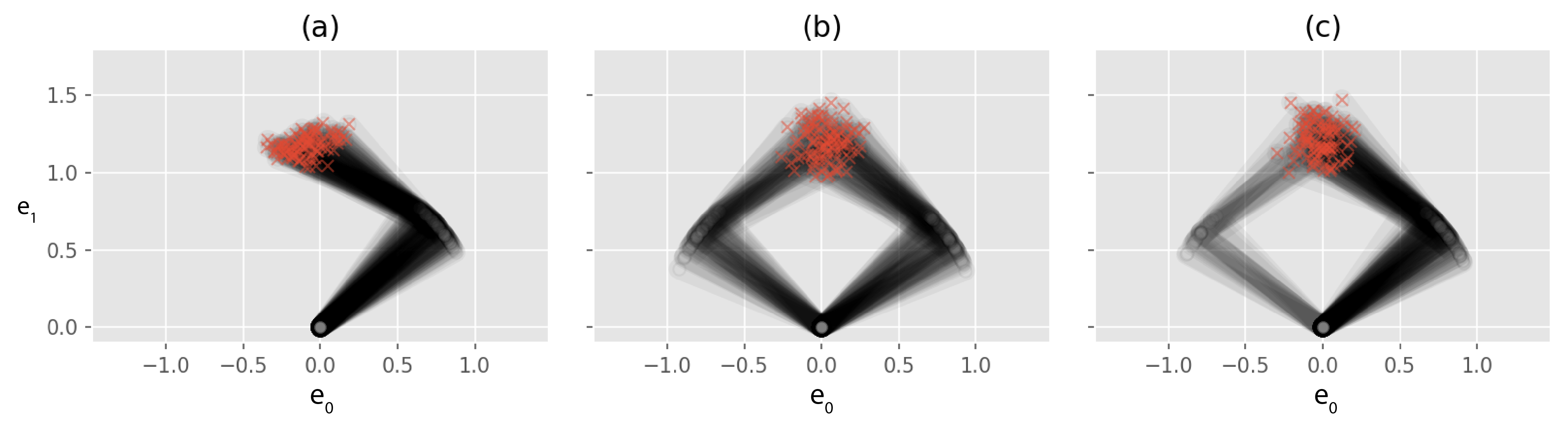
Figure 3: The product of experts is an unnormalized density. As in Fig. 2, the density shown in (a) results from an elongated Gaussian defined on the end-effector of a 2-DoF planar robot. For control applications, such as keeping the robot in this distribution, accessing the unnormalized density is sufficient. For other applications, such as training a PoE, sampling from this distribution, evaluating the normalizing constant and its gradient might be needed. Using variational inference, the PoE can be approximated by a tractable distribution, as a mixture of banana-shaped distributions (b) or Gaussians (c). On purpose, only 5 mixture components were used in the illustrations. A more precise approximation can be achieved with a higher number.
Learning compares expert statistics on demonstrated configurations with statistics under the model. Contrastive divergence approximates the latter using short data-initialized chains; the proposed method alternates fitting a variational mixture and updating expert parameters. Importance weights reduce approximation bias, and optional sampling refinements improve robustness.
Experts with tractable likelihoods are first fitted independently. Those fits initialize the subsequent joint learning, reducing the search burden without replacing product normalization.
3 Product of Experts with nullspace filter (PoENS)
PoENS projects secondary expert gradients into the primary task’s Jacobian null space. This prevents secondary updates from directly changing the protected task directions and helps explain why a desired secondary goal was not reached.
Unlike an ordinary PoE, this construction is supplied as a filtered gradient field, without an evaluated scalar log-density. The paper uses stochastic variational updates compatible with that field. Its examples support the proposed approximation; they are not a general proof that arbitrary filtered fields define a normalized density.
Equations 17–21
(17)
(18)
(19)
(20)
(21)
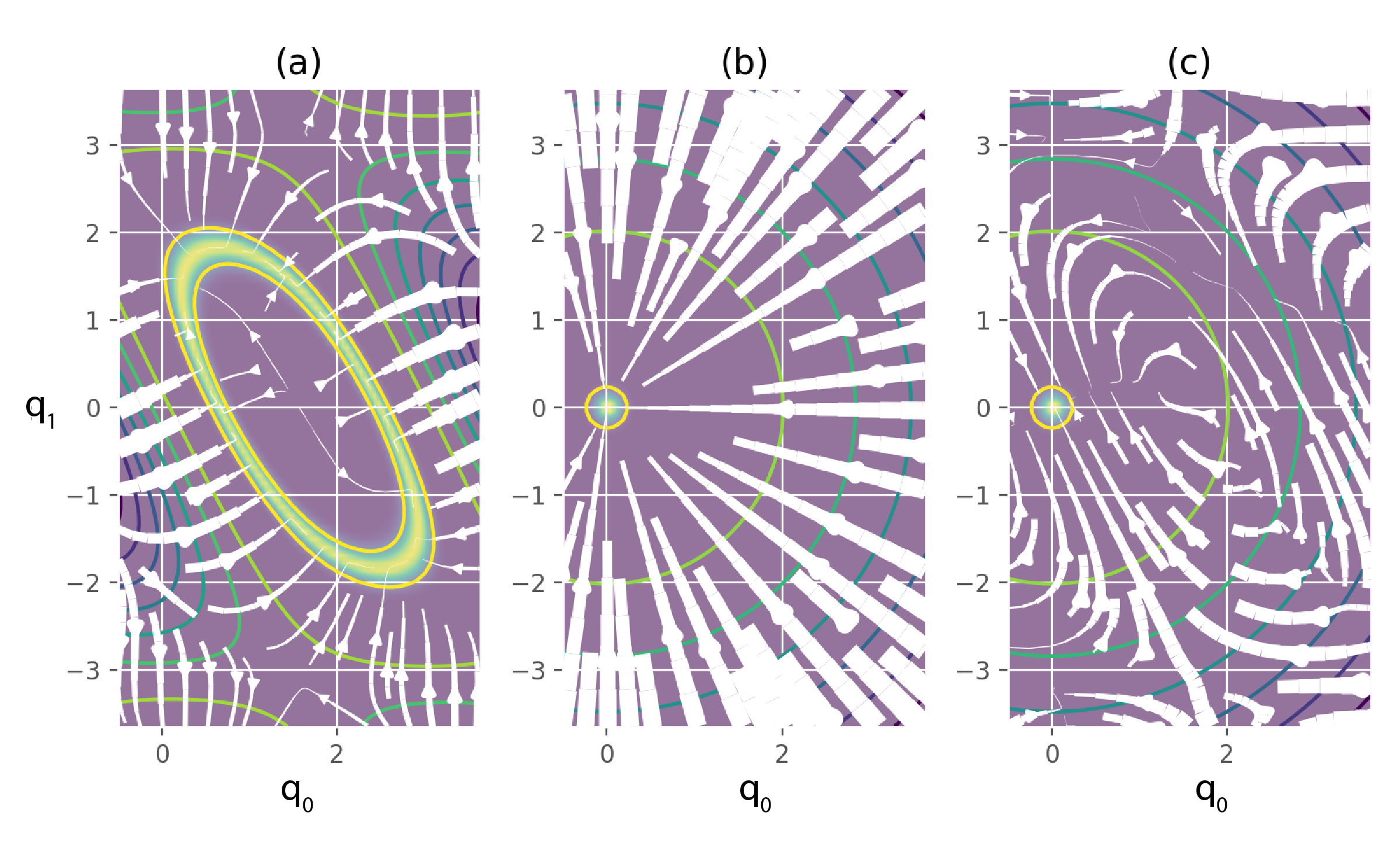
Figure 4: Densities and derivatives of a two-expert problem. A 2-DoF planar robot is considered as in Fig. 2. The first expert is an elongated Gaussian distribution on its end-effector. The second expert acts in joint angles and defines a preferred configuration. (a) The density of the expert is shown as a colormap. The derivative is displayed as streamlines.
(b) The same is done with the second objective in configuration space.
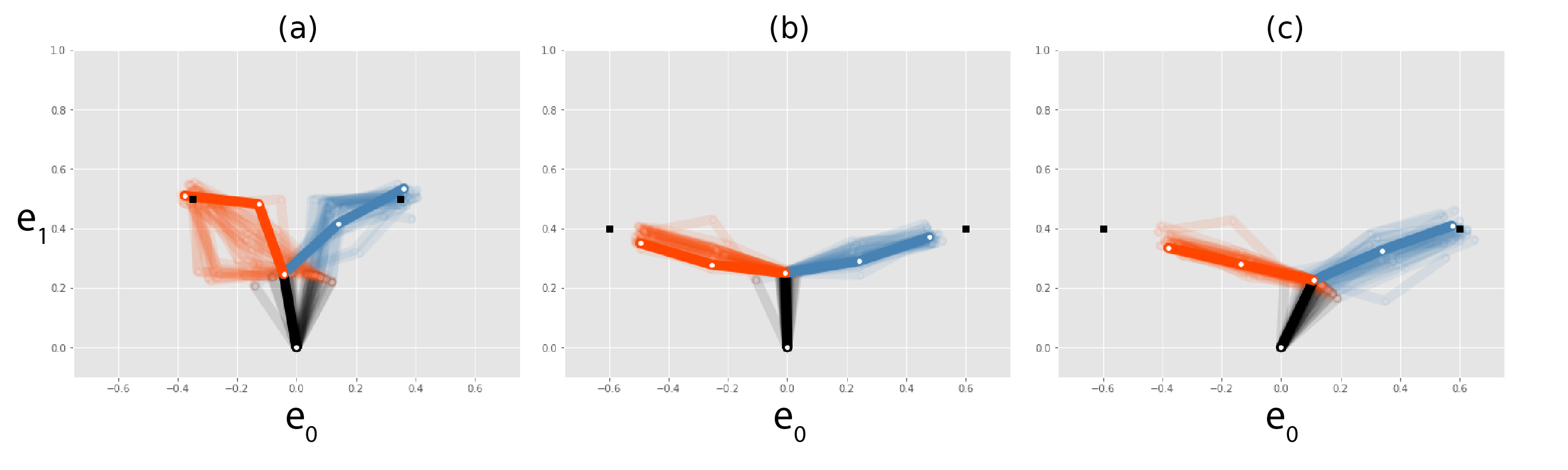
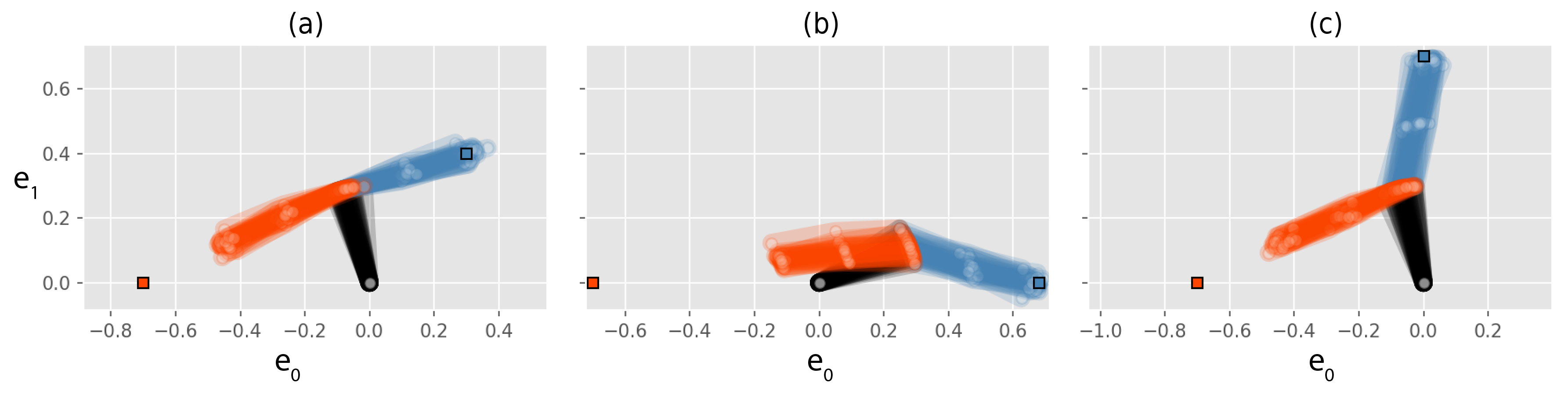
(c) The derivative of the second experts is this time filtered as . Figure 5: 5-DoF bimanual planar robot with two forward kinematics objectives. Variational inference is used to generate the displayed samples. (a) The two tasks are compatible and the distribution of solution is approximated. (b) No nullspace, the two tasks are of the same importance. (c) The gradient of the objective of the orange arm is projected onto the nullspace of the Jacobian of the forward kinematics of the blue arm. This is achieved with stochastic variational inference that only requires to evaluate the gradient of the unnormalized density.
4 Useful distributions and transformations for robotics
The following toolkit supplies transformations and expert scores for common robotic constraints.
4.1 Transformations
Transformations may be known from kinematics, partly unknown, or learned. Joint training can estimate transformation parameters together with expert preferences.
Forward kinematics maps joints into link poses, possibly relative to an object. Unknown object frames or a held tool’s fixed offset can be learned when they provide a compact explanation of demonstrated configurations.
Equation 22
(22)
Manipulability
Manipulability descriptors encode directions in which motion or force is easy. Their physically attainable values depend on kinematics and higher-priority tasks. Joint learning can account for that restricted support instead of treating every mathematical matrix as attainable.
Equations 23–24
(23)
(24)
Relative distances
Distances between robot points and targets or obstacles offer an alternative task representation. They can complement pose constraints in cluttered environments.
Link masses and kinematics determine the center of mass. For static equilibrium on level ground, its projection should lie within the support polygon.
Jacobian pseudoinverse iterations
Repeated Jacobian-pseudoinverse corrections can be included inside a transformation to approximate very tight constraints. This improves concentration near a solution manifold but can bias mass toward locally linear regions and adds differentiation cost.
Equations 25–28
(25)
(26)
(27)
(28)
Neural network
Invertible neural transformations can map complex demonstrated shapes to simple expert distributions. Change-of-variable likelihoods provide initialization, while regularizing the inverse Jacobian discourages abrupt distortion. A diffeomorphism preserves the underlying expert’s isolated optimum; the full multi-expert robot problem can still have multiple solutions.
Equations 29–30
(29)
(30)
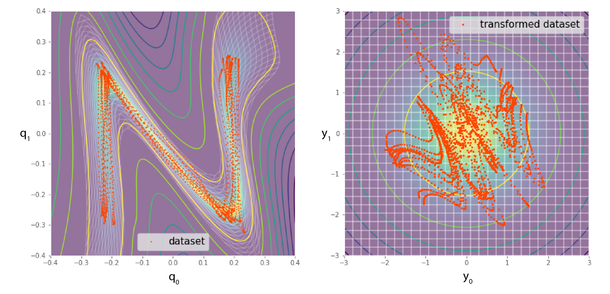
Figure 6: For greater expressiveness, an invertible neural network can be used as an expert transformation . Instead of optimizing the parameters of the expert density , which can be set as a zero-centered and unit covariance Gaussian (right), the parameters of the network can be trained. The neural network becomes a transformation under which the dataset (N shape, left) becomes a simple distribution (Gaussian, right). The densities are shown as a colormap with isolines. A grid that undergoes the inverse transformation is also shown. This approach allows complex attractors or guiding distributions to be learned, where it is easy to control the robot in the transformed space.
4.2 Distributions
Different expert families express point targets, orientations, trajectories, inequality constraints, and optional objectives.
Gaussian experts have quadratic negative log-likelihoods, making them convenient for inverse kinematics and quadratic control. Their covariance determines directional precision.
Matrix Bingham–von Mises–Fisher scores describe rotations without requiring a separate orientation normalizer. Structured quadratic forms can couple positions and vectorized rotation matrices, with positive-definiteness constraints controlling valid covariance parametrizations.
Equations 32–36
(32)
(33)
(34)
(35)
(36)
Matrix normal distribution
Matrix-normal experts reduce parameter count by separating row and column covariance. They are useful when a transformation naturally produces a matrix.
Equations 37–38
(37)
(38)
Probabilistic movement primitives
ProMP experts extend the framework from static configurations to trajectory distributions. A mixture of joint-space ProMPs can approximate products involving task-space and joint-space trajectories, including multiple kinematic solution families. [47]
Equations 39–40
(39)
(40)
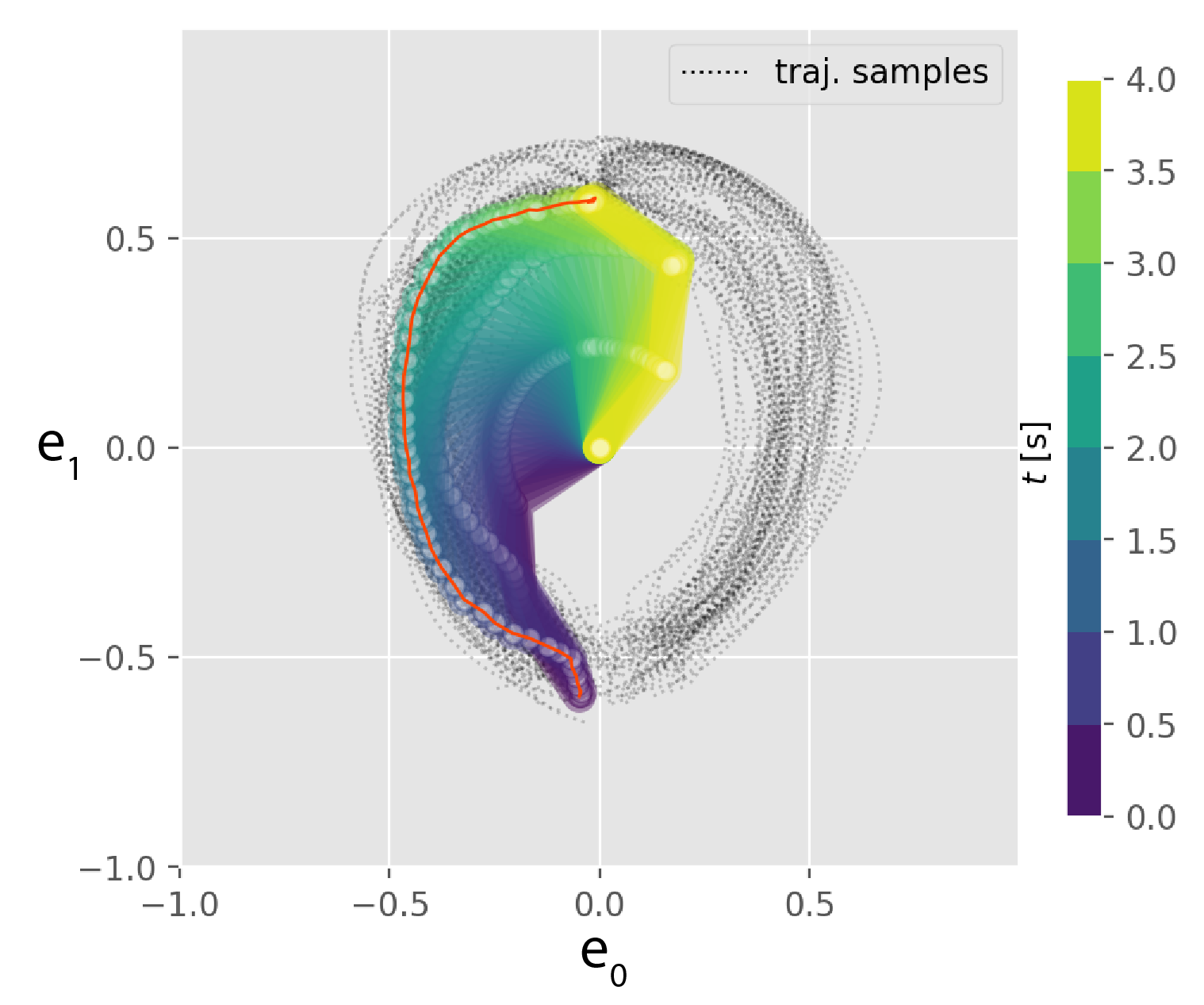
Figure 7: To encode distributions of trajectories, probabilistic movement primitives (ProMP) can be used as experts in a PoE. In this example, a product of two ProMP experts is considered: one defines a joint angle trajectory, while the other defines the trajectory of the end-effector. A 3-DoF planar robot is used in this example. The product of ProMPs is approximated using variational inference as a mixture of ProMPs in configuration space. Samples of trajectories of the end-effector are displayed, as well as a full sequence of configurations. Even if each expert is Gaussian, the product of ProMPs is multimodal because of the planar robot kinematics.
Approximate distributions in the tangent space of manifolds
Gaussian scores in a manifold’s tangent space offer a generic treatment of orientations and other geometric data. The logarithmic map must be differentiable for the proposed training procedure.
Cumulative Gaussian probabilities provide smooth inequality scores for joint limits, obstacles, and equilibrium. Their scale controls the transition margin. These probabilistic penalties alone are not hard safety guarantees.
Equation 42
(42)
Uni-Gauss distributions
A uniform–Gaussian mixture allows an objective to be effectively inactive. It gives softer prioritization than null-space projection. Enumerating active-task combinations is practical only for small task sets; marginalized mixtures avoid that combinatorial expansion.
Equation 43
(43)
5 Control
One controller seeks and maintains high-density configurations. Another plans motion whose spatial coverage approximates the desired distribution.
5.1 Optimal control
LQT augments the robot state with expert task coordinates and linearizes their dynamics. Gaussian expert costs become quadratic; other scores require local approximation. Learned precision sets feedback strength, allowing compliance in unconstrained directions.
A slower loop recomputes the controller in 2–10 milliseconds, while a faster loop executes the latest command in under one millisecond in the reported implementation. Both algorithms and the disturbance-response example are preserved.
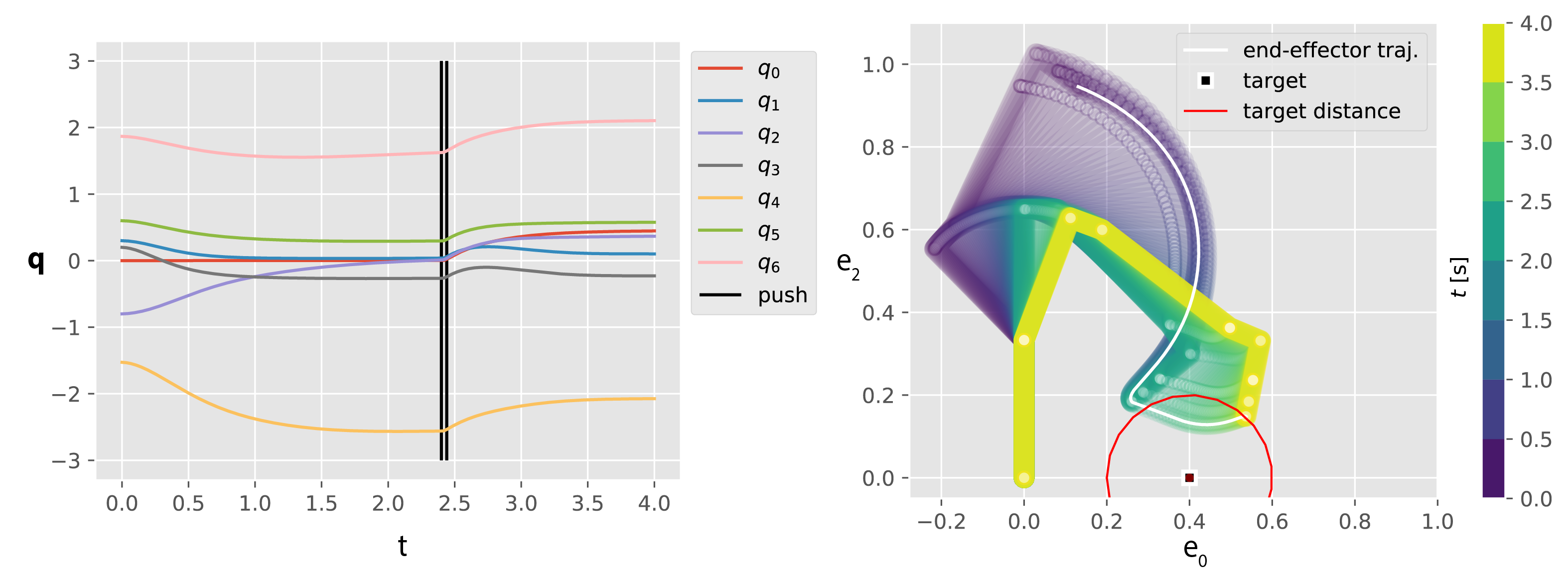
Figure 8: Example of 7-DoF manipulator controlled with an LQT. To show the time evolution, only the kinematic chain is displayed. The PoE is the intersection between a vertical plane () and a sphere. The two experts act on the end-effector. They are defined by a Gaussian distribution on around and by a Gaussian distribution on the log-distance to a target (black square). On the left, the evolution of the values of the joint angles is displayed over time. At , a perturbation in configuration space occurs. The robot converges to a new local mode of the PoE.
5.2 Ergodic control
Ergodic control instead matches the trajectory’s time-averaged coverage to the target density. A mixture around trajectory points models sensing or influence radius; velocity and acceleration penalties make the path executable. The same variational objective supports optimization without a normalized target.
Equations 59–60
(59)
(60)
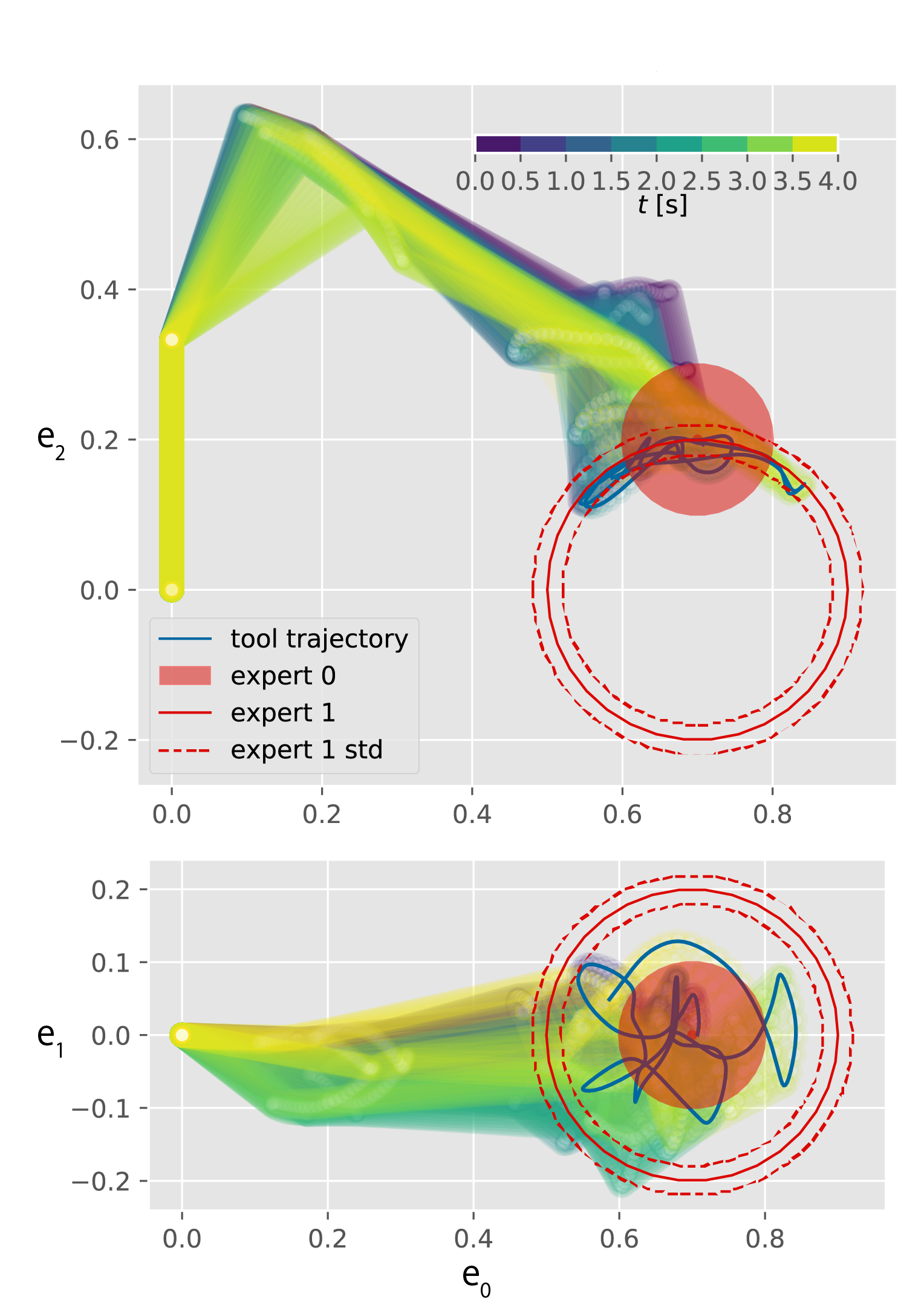
Figure 9: The trajectory of the robot is optimized to cover the PoE. The density is defined by a position constraint of the end-effector (expert 0) and a distance constraint (expert 1).
6 Experiments
The experiments test density estimation, hidden priorities, learned task transformations, and pose correlations. Distribution discrepancy is the main quantitative metric; it is not a task-success percentage.
6.1 Multimodal distributions
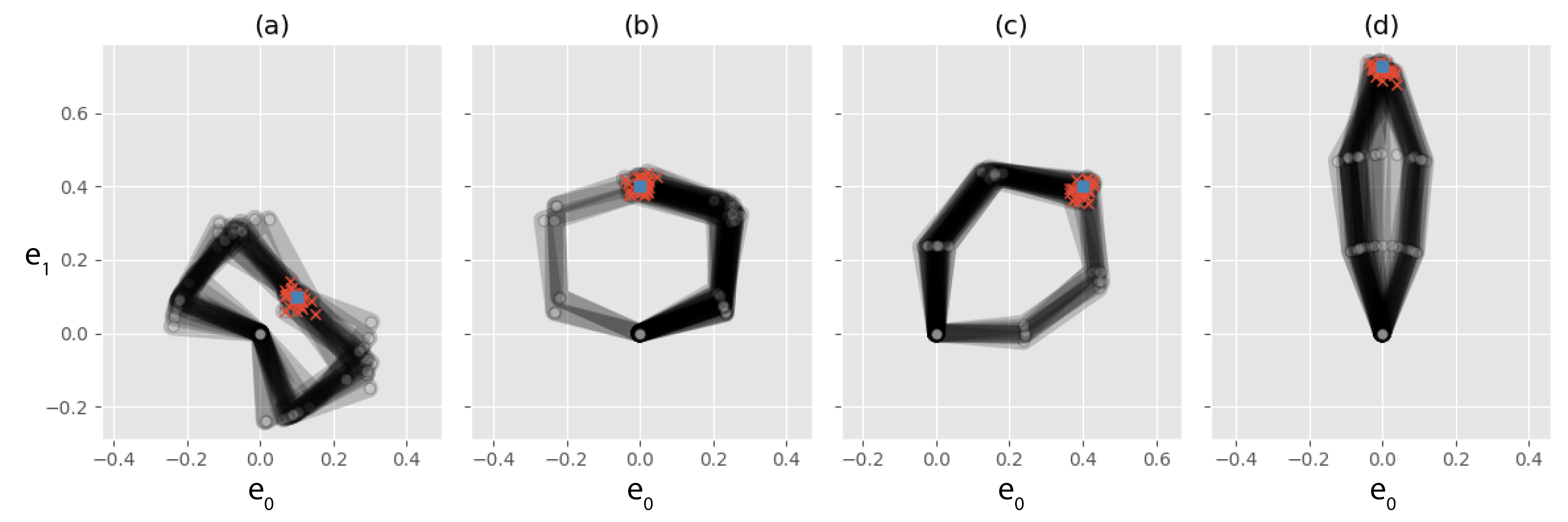
Three two-joint planar datasets contain thirty configurations each. Across random initializations, variational learning gives lower alpha-divergence than contrastive divergence: 0.067 versus 0.837 for the joint-target case, 0.016 versus 0.039 for the task-target case, and 0.014 versus 0.063 for their combination. Missing alternative kinematic modes explains much of the sampling baseline’s error.
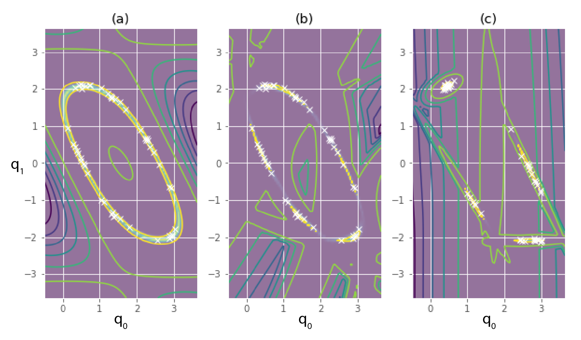
Figure 10: Samples of configurations for three tasks that illustrate the advantages of using variational inference with a mixture model for training a PoE. A 2-DoF planar robot is considered. (a) Joint angle target. (b) Operational space target (c) Operational space target and joint angle target. Equations 61
(61)
Table 1: Quantitative evaluations of the learned distribution using contrastive divergence (CD) and our approach based on variational inference with a Gaussian mixture model (VI). The table shows alpha-divergence measures between the different approximations and the ground-truth distribution, computed for the three tasks shown in Fig. 10.
These tests ask whether a model can recover a secondary target that demonstrations cannot satisfy because a primary objective takes precedence.
Planar robot
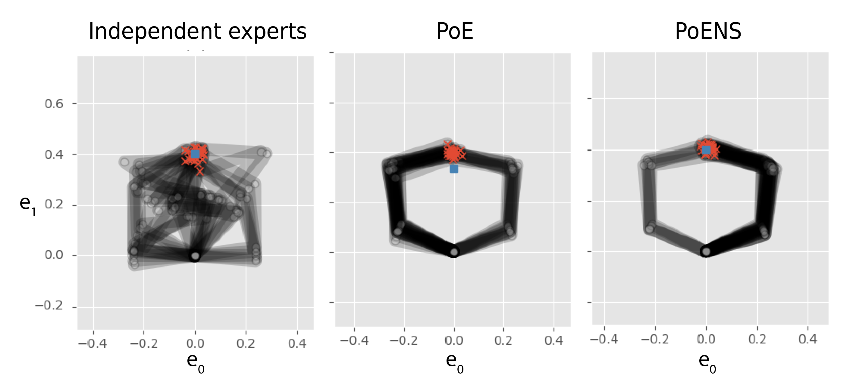
Planar bimanual reaching uses thirty samples for each of three primary targets. A separate three-joint test combines reaching with manipulability, using four target conditions. Providing the hierarchy lets PoENS recover goals more accurately than independent fits or an unprioritized product.
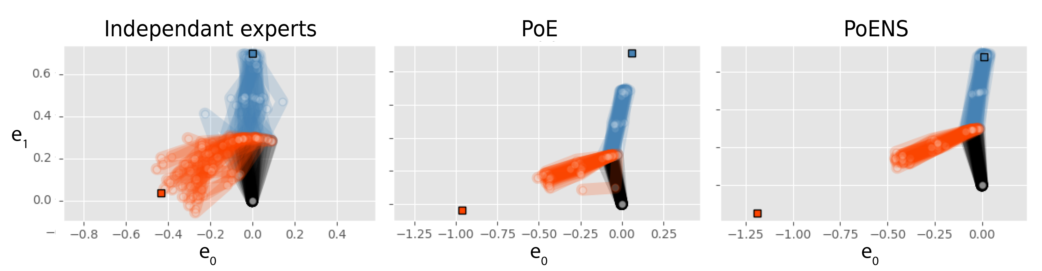
Table 2 reports alpha-divergence 0.094 for bimanual PoENS versus 0.258 for PoE and 1.814 for independent experts; corresponding manipulability values are 0.202, 0.630, and 0.812. The scalar manipulability comparison simplifies the richer baseline representation.
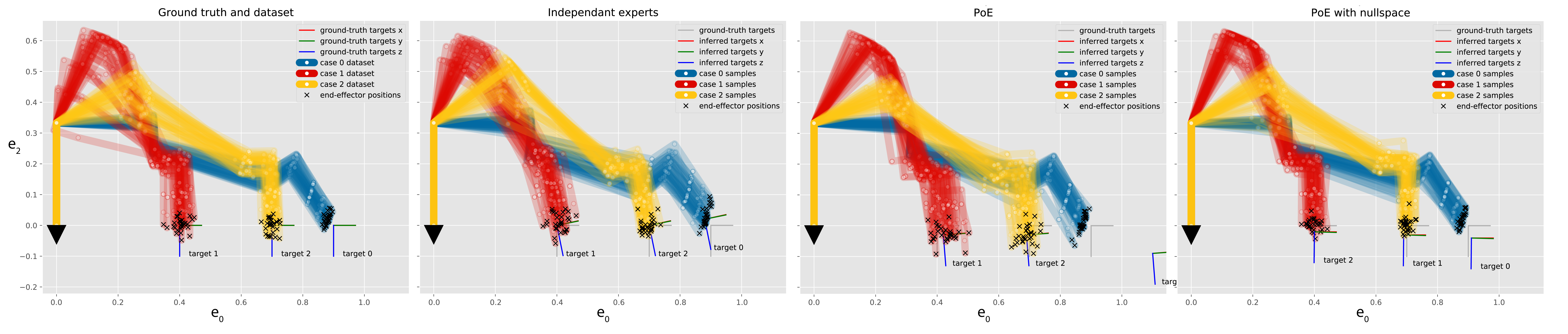
Figure 11: Dataset for the bimanual task with a hierarchy. Three situations are given, where each end-effector should track the target of the same color (displayed as a square).Figure 12: Samples from the different models learned for the bimanual task with a hierarchy. Left: Using independent experts, the secondary task is not well understood and its variance is over-estimated. Center: Using a PoE, the target of the primary task is inferred to be further away. Right: Using a PoE with a nullspace structure, the targets are well recovered.Equation
Figure 13: Dataset for the hierarchical task with a manipulability objective. The robot should track the target (displayed as a blue square) and maximize a manipulability measure. Four different targets are given.Equation
Figure 14: Samples from the different models learned for the task with a manipulability objective. Left: Using independent experts, the secondary task is not well understood (the manipulability measure has a big variance in the dataset). Center: Using a PoE, the estimation of the principal objective is biased. Right: By providing the hierarchical structure, the two objectives are well understood.
Table 2: Quantitative evaluations of the quality of the learned distribution for the two planar tasks. The table shows alpha-divergence measures between the different approximations and the ground-truth distribution are computed. (a) Bimanual task (b) Manipulability objective
The Panda welding-like dataset prioritizes end-effector position over a preferred vertical orientation, with thirty configurations in each of three target conditions. PoENS gives the lowest reported discrepancy in all three. Unbiased squared-MMD estimates may be slightly negative near zero; these are estimator fluctuations, not negative distances.
Equation
Table 3: Quantitative evaluations of the quality of the learned distribution for the 7-DoF Panda robot (welding task). The table shows maximum mean discrepancy measures between the dataset and different models for the 3 cases displayed in Fig. 17.
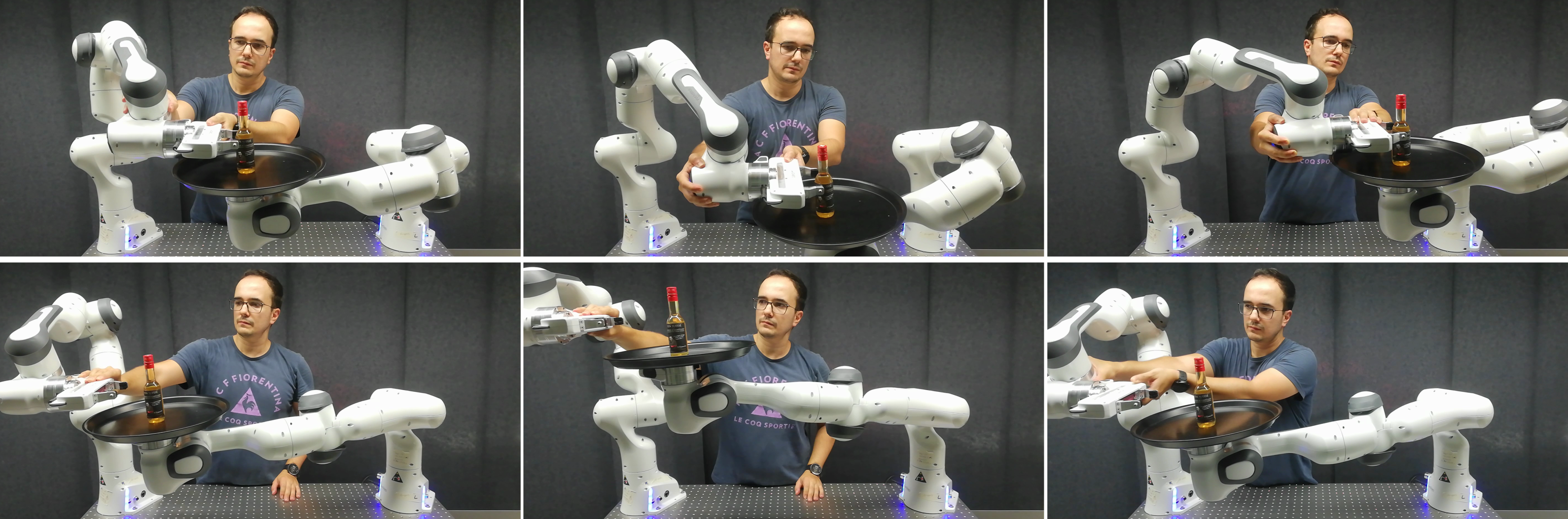
In physical tray serving, the robot prioritizes a level tray over placing a bottle within the other gripper. Ten samples in each of three hand-position conditions teach both target relationships and priority. A second gravity-compensated robot stands in for the person. The demonstration shows compliant reproduction, without reporting a large-scale success-rate evaluation.
Figure 15: Several demonstrations of the desired priority behavior are given.Top: Both position and orientation are achievable. Bottom: Position is only partially fulfilled, to allow the tray to remain parallel to the floor. The left robot arm is playing the role of a person who should grasp the bottle.Figure 16: The right arm should keep the tray horizontal and the bottle between the gripper fingers. With a PoENS model, the robot learns i) the tray pose with respect to the gripper and ii) that the tray orientation has a higher priority than the position. Top row: Reproduction when both position and orientation can be fulfilled. Bottom row: Reproduction when position reference is too far so the robot prioritizes orientation.Figure 17: Dataset and retrieved samples for the hierarchical task with the 7-DoF Panda robot (welding task). Only the kinematic chain of the robot is displayed, such that multiple samples can be shown. The dataset provides three different situations (displayed in blue, yellow and red) in which the robot should track a different target with its end-effector. In each situation, the orientation should be held vertical as a secondary task.
Further experiments estimate partly unknown transformations and test whether explicit kinematic structure reduces sample requirements.
New end-effector
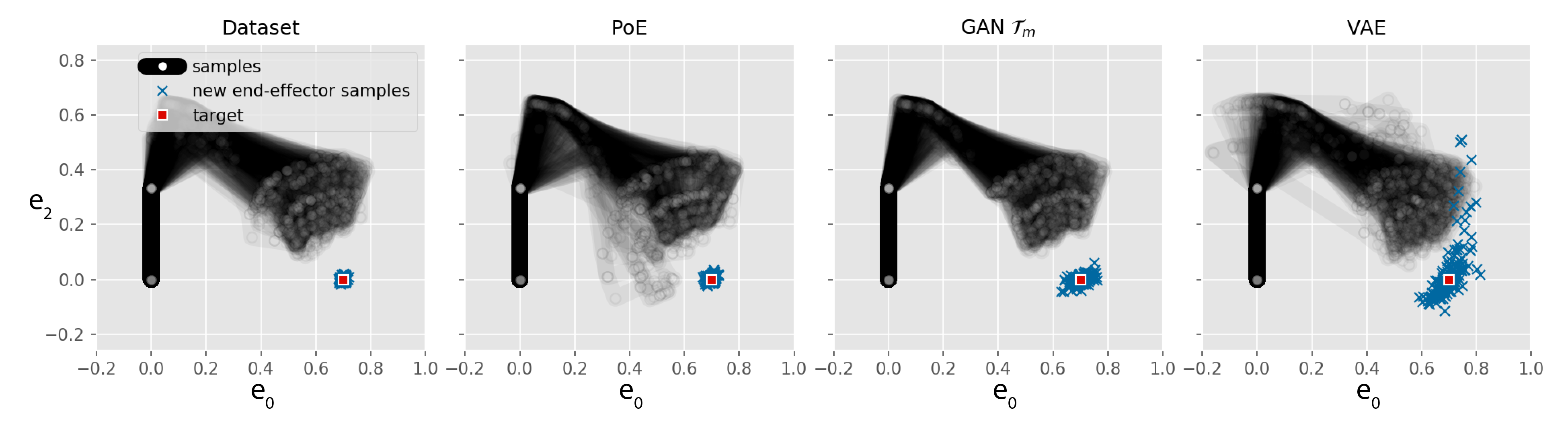
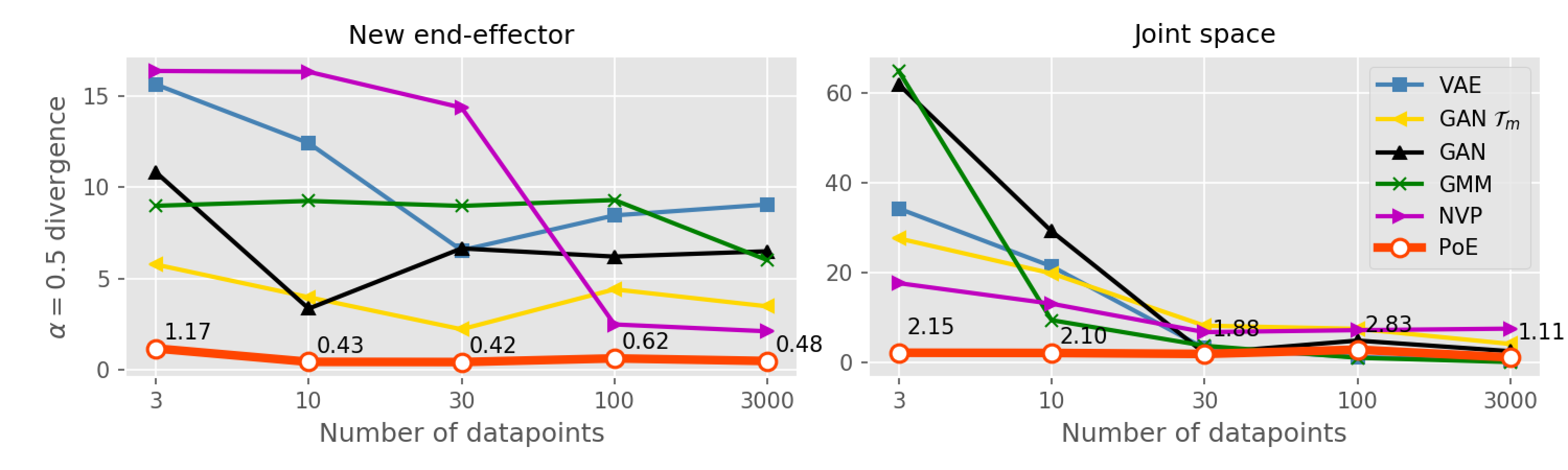
A seven-joint Panda learns the offset of a new tool and its target distribution from datasets of 3, 10, 30, 100, or 3,000 configurations. The paper compares PoE with a VAE, mixture model, invertible network, and two GAN variants. Structured PoE performs best in the reported distribution comparisons; task-space features also help the GAN.
The text describes this evaluation as squared MMD, while Figure 19’s caption calls it alpha-divergence. That inconsistency limits interpretation of the plotted metric label.
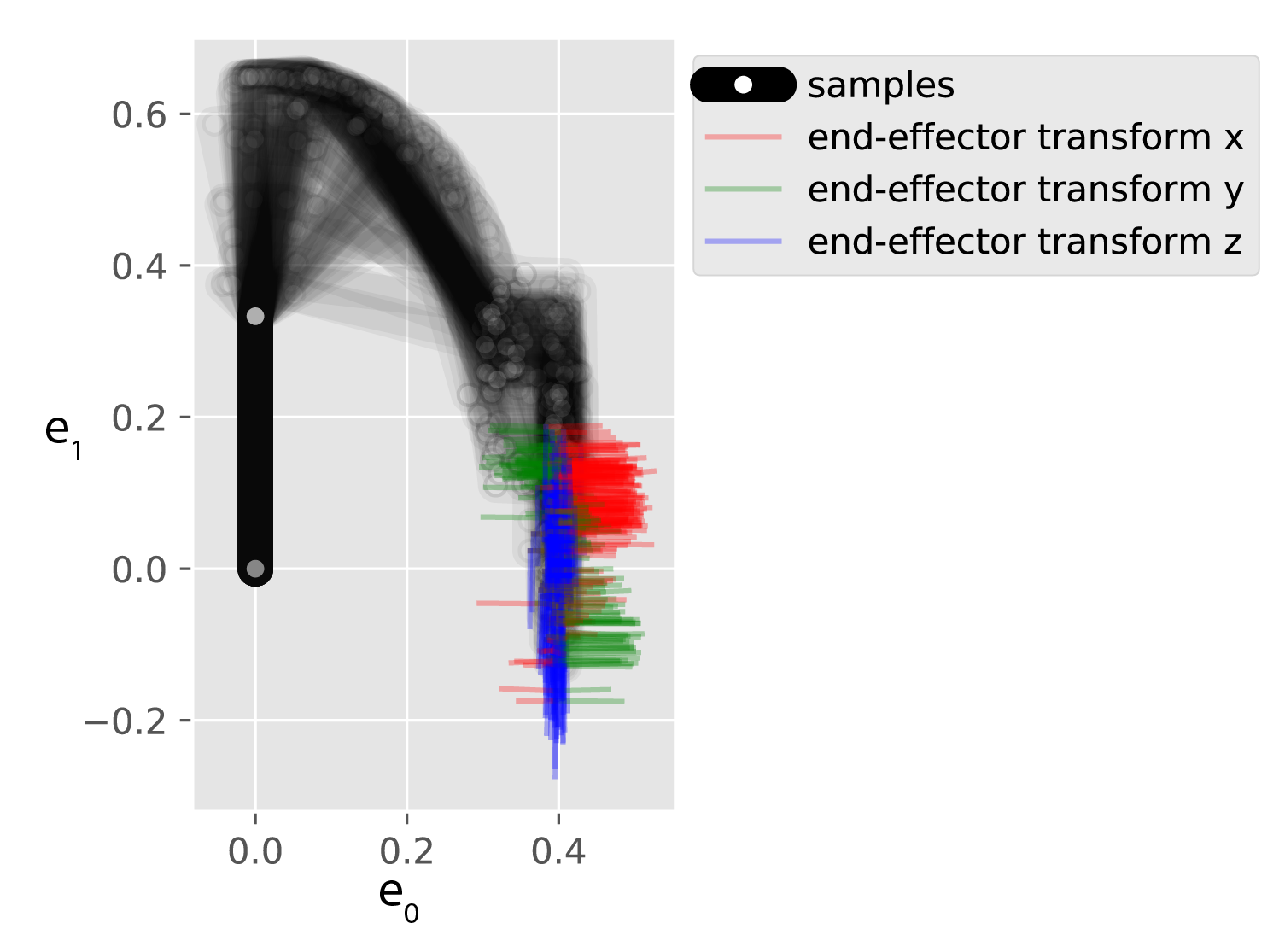
Figure 18: Dataset and samples from the different models for a task involving an unknown end-effector. In this illustration, the models were trained with 3000 samples.Equation
Figure 19: Quantitative results for a task involving an unknown end-effector. The graphs show alpha-divergence measures (with ) between the dataset and the different models for the different sizes of the dataset.
Conditional distributions
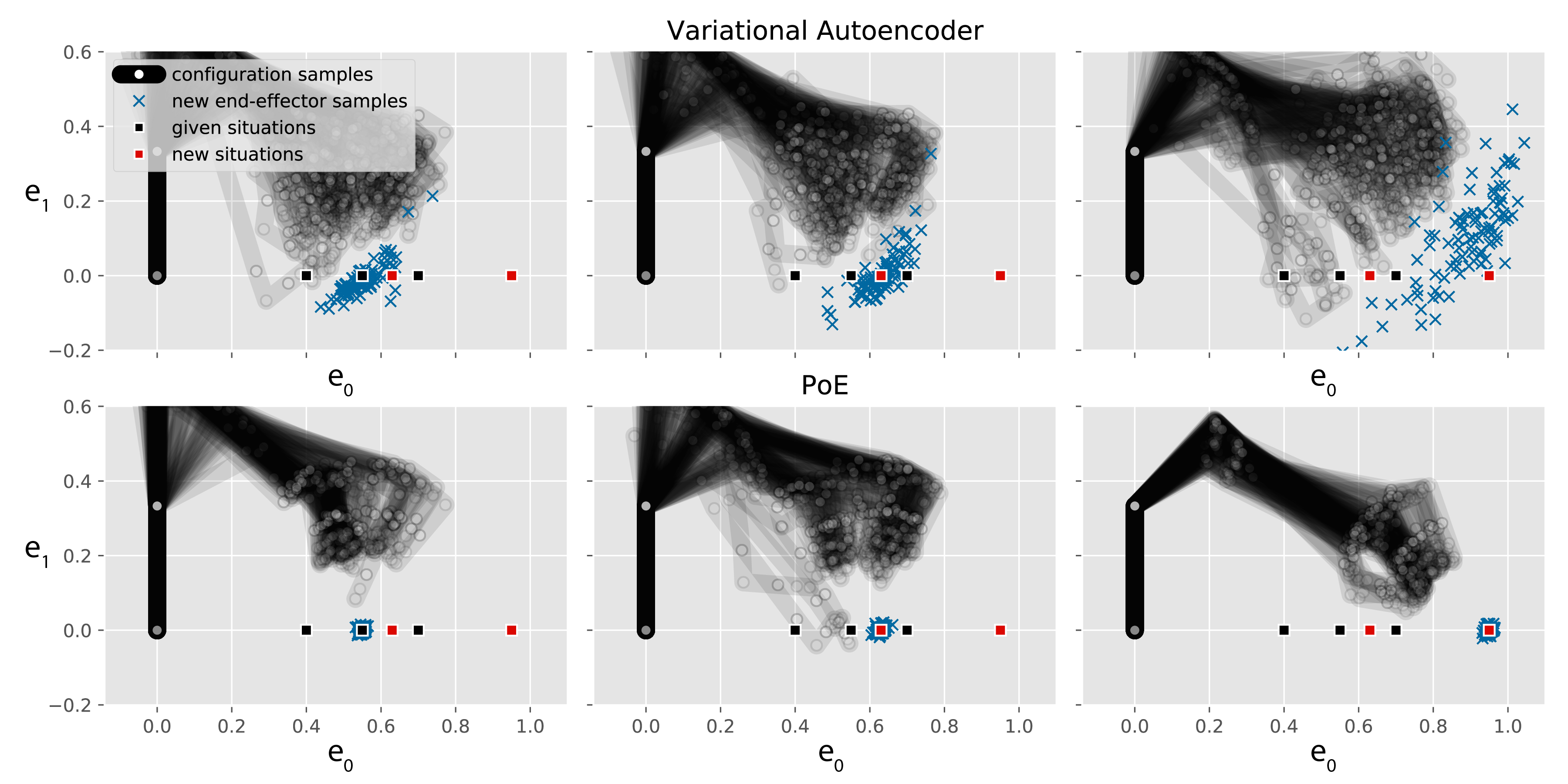
Conditional learning uses three known targets with 1,000 configurations each. PoE transfers to a seen, interpolated, and distant target with much lower reported discrepancy than the VAE and GMR baselines. Sampling a new PoE condition requires a fresh approximation; evaluating its unnormalized control cost does not.
Figure 20: Dataset and samples from the different models for a task involving an unknown end-effector. Three cases are reproduced. Left column: The distribution is sampled on a known target. Middle column: The target is in-between two given targets. Right column: The target is far from the given targets. The first and second rows show results for a conditional variational autoencoder and a PoE, respectively.Equation
Table 4: Quantitative results for the task with the new end-effector. The table shows maximum mean discrepancy measures between the dataset and the different models for the different cases. (a) The distribution is sampled on a known target. (b) The target is in-between two given targets. (c) Generalization with respect to a new target far from the given targets.
6.4 End-effector position and rotation correlations
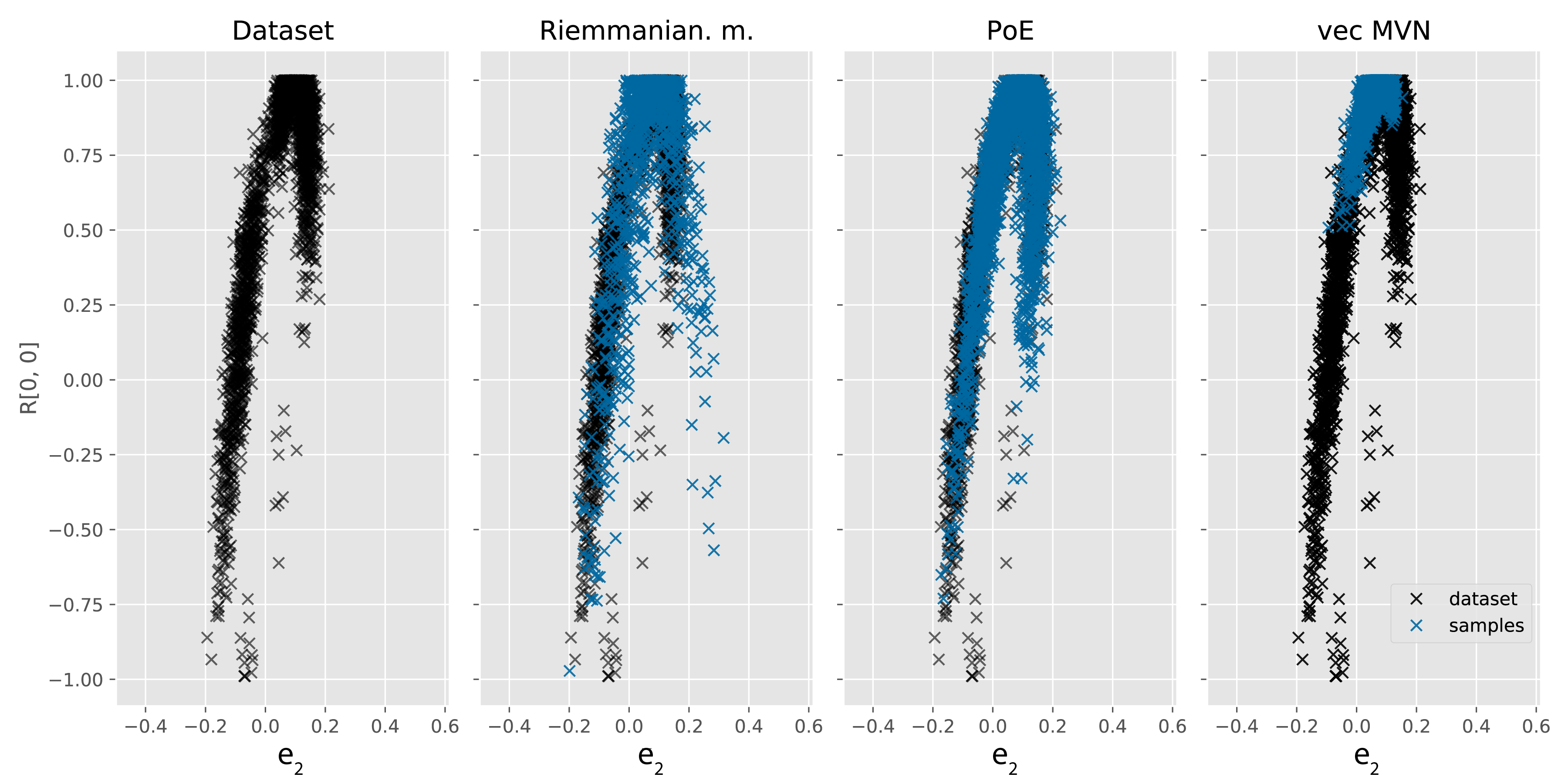
Three synthetic datasets of 3,000 configurations couple end-effector height and orientation. The model uses a twelve-dimensional pose representation with diagonal plus rank-one covariance. It compares against independently fitted vectorized Gaussians and a Riemannian representation.
PoE has the highest reported test p-values and the lowest squared MMD in cases (b) and (c). In case (a), Table 5 gives the Riemannian model a smaller MMD, 0.00103 versus 0.0015, despite the prose claiming PoE wins every case. The preserved table supports this narrower conclusion.
Figure 21: Samples where the height of the end-effector is correlated with its rotation along the -axis. The transformation matrix of the end-effector is displayed.Equation
Figure 22: Scatter plot showing the correlation between the height of the end-effector and the first element of the first row of the rotation matrix for case (a). The dataset is shown in black and the samples from the different models in blue.
Table 5: Quantitative results for the task with a correlation between position and orientation. The table shows and maximum mean discrepancy measures between the dataset and the different models for the different cases.
Jointly normalized expert models exploit robot structure to learn useful constraints from small datasets, while null-space filtering helps recover masked secondary goals. Results support the studied tasks and model families. Expressive learned transformations and broader robotics applications remain directions for extending the framework.
69 references
[Abadi et al.(2016)Abadi, Barham, Chen, Chen, Davis, Dean, Devin,
Ghemawat, Irving, Isard, Kudlur, Levenberg, Monga, Moore, Murray, Steiner,
Tucker, Vasudevan, Warden, Wicke, Yu and Zheng]Abadi M, Barham P, Chen J, Chen Z, Davis A, Dean J, Devin M, Ghemawat S, Irving G, Isard M, Kudlur M, Levenberg J, Monga R, Moore S, Murray DG, Steiner B, Tucker P, Vasudevan V, Warden P, Wicke M, Yu Y and Zheng X (2016) Tensorflow: A system for large-scale machine learning.In: 12th USENIX Symposium on Operating Systems Design and
Implementation (OSDI 16). pp. 265–283.
[Amato and Wu(1996)]Amato NM and Wu Y (1996) A randomized roadmap method for path and manipulation planning.In: Proc. IEEE Intl Conf. on Robotics and Automation
(ICRA), volume 1. IEEE, pp. 113–120.
[Andrieu et al.(2003)Andrieu, De Freitas, Doucet and
Jordan]Andrieu C, De Freitas N, Doucet A and Jordan MI (2003) An introduction to mcmc for machine learning.Machine learning 50(1-2): 5–43.
[Arenz et al.(2018)Arenz, Neumann and Zhong]Arenz O, Neumann G and Zhong M (2018) Efficient gradient-free variational inference using policy search.In: Proc. Intl Conf. on Machine Learning (ICML),
volume 80. PMLR, pp. 234–243.
[Ayvali et al.(2017)Ayvali, Salman and Choset]Ayvali E, Salman H and Choset H (2017) Ergodic coverage in constrained environments using stochastic trajectory optimization.In: Proc. IEEE/RSJ Intl Conf. on Intelligent Robots and
Systems (IROS). IEEE, pp. 5204–5210.
[Bengio et al.(2014)Bengio, Laufer, Alain and
Yosinski]Bengio Y, Laufer E, Alain G and Yosinski J (2014) Deep generative stochastic networks trainable by backprop.In: Proc. Intl Conf. on Machine Learning (ICML). pp.
226–234.
[Berenson et al.(2011)Berenson, Srinivasa and
Kuffner]Berenson D, Srinivasa S and Kuffner J (2011) Task space regions: A framework for pose-constrained manipulation planning.The International Journal of Robotics Research 30(12):
1435–1460.
[Bishop et al.(1998)Bishop, Lawrence, Jaakkola and
Jordan]Bishop CM, Lawrence ND, Jaakkola T and Jordan MI (1998) Approximating posterior distributions in belief networks using mixtures.In: Advances in Neural Information Processing Systems
(NIPS). pp. 416–422.
[Bohner and Wintz(2011)]Bohner M and Wintz N (2011) The linear quadratic tracker on time scales.International Journal of Dynamical Systems and Differential
Equations 3(4): 423–447.
[Calinon and Billard(2009)]Calinon S and Billard A (2009) Statistical learning by imitation of competing constraints in joint space and task space.Advanced Robotics 23(15): 2059–2076.
[Chen et al.(2014)Chen, Fox and Guestrin]Chen T, Fox E and Guestrin C (2014) Stochastic gradient Hamiltonian monte carlo.In: Proc. Intl Conf. on Machine Learning (ICML). pp.
1683–1691.
[Dempster et al.(1977)Dempster, Laird and Rubin]Dempster AP, Laird NM and Rubin DB (1977) Maximum likelihood from incomplete data via the em algorithm.Journal of the Royal Statistical Society: Series B
(Methodological) 39(1): 1–22.
[Dinh et al.(2017)Dinh, Sohl-Dickstein and Bengio]Dinh L, Sohl-Dickstein J and Bengio S (2017) Density estimation using Real NVP.In: Proc. Intl Conf. on Learning Representation(ICLR).
[Duane et al.(1987)Duane, Kennedy, Pendleton and
Roweth]Duane S, Kennedy AD, Pendleton BJ and Roweth D (1987) Hybrid Monte Carlo.Physics letters B 195(2): 216–222.
[Finn et al.(2016)Finn, Levine and Abbeel]Finn C, Levine S and Abbeel P (2016) Guided cost learning: Deep inverse optimal control via policy optimization.In: Proc. Intl Conf. on Machine Learning (ICML). pp.
49–58.
[Goodfellow et al.(2014)Goodfellow, Pouget-Abadie, Mirza, Xu,
Warde-Farley, Ozair, Courville and Bengio]Goodfellow I, Pouget-Abadie J, Mirza M, Xu B, Warde-Farley D, Ozair S, Courville A and Bengio Y (2014) Generative adversarial nets.In: Advances in Neural Information Processing Systems
(NIPS). pp. 2672–2680.
[Gretton et al.(2012)Gretton, Borgwardt, Rasch, Schölkopf and
Smola]Gretton A, Borgwardt KM, Rasch MJ, Schölkopf B and Smola A (2012) A kernel two-sample test.Journal of Machine Learning Research 13(Mar): 723–773.
[Guo et al.(2016)Guo, Wang, Fan, Broderick and
Dunson]Guo F, Wang X, Fan K, Broderick T and Dunson DB (2016) Boosting variational inference.Advances in Neural Information Processing Systems (NIPS) .
[Hinton et al.(2006)Hinton, Osindero and Teh]Hinton GE, Osindero S and Teh YW (2006) A fast learning algorithm for deep belief nets.Neural computation 18(7): 1527–1554.
[Ichter et al.(2018)Ichter, Harrison and Pavone]Ichter B, Harrison J and Pavone M (2018) Learning sampling distributions for robot motion planning.In: Proc. IEEE Intl Conf. on Robotics and Automation
(ICRA). IEEE, pp. 7087–7094.
[Jaquier et al.(2020)Jaquier, Rozo, Caldwell and
Calinon]Jaquier N, Rozo L, Caldwell DG and Calinon S (2020) Geometry-aware manipulability learning, tracking and transfer.International Journal of Robotics Research (IJRR) .
[Jetchev and Toussaint(2011)]Jetchev N and Toussaint M (2011) Task space retrieval using inverse feedback control.In: Proc. Intl Conf. on Machine Learning (ICML). pp.
449–456.
[Johnson et al.(2017)Johnson, Keller and
Weintraut]Johnson DD, Keller RM and Weintraut N (2017) Learning to create jazz melodies using a product of experts.In: International Conference on Computational Creativity. pp.
151–158.
[Kalakrishnan et al.(2013)Kalakrishnan, Pastor, Righetti and
Schaal]Kalakrishnan M, Pastor P, Righetti L and Schaal S (2013) Learning objective functions for manipulation.In: Proc. IEEE Intl Conf. on Robotics and Automation
(ICRA). IEEE, pp. 1331–1336.
[Khatri and Mardia(1977)]Khatri C and Mardia K (1977) The von Mises-Fisher matrix distribution in orientation statistics.Journal of the Royal Statistical Society. Series B
(Methodological) : 95–106.
[Kopicki et al.(2017)Kopicki, Zurek, Stolkin, Moerwald and
Wyatt]Kopicki M, Zurek S, Stolkin R, Moerwald T and Wyatt JL (2017) Learning modular and transferable forward models of the motions of push manipulated objects.Autonomous Robots 41(5): 1061–1082.
[Kume et al.(2013)Kume, Preston and Wood]Kume A, Preston S and Wood AT (2013) Saddlepoint approximations for the normalizing constant of Fisher–Bingham distributions on products of spheres and stiefel manifolds.Biometrika 100(4): 971–984.
[Lehner and Albu-Schäffer(2017)]Lehner P and Albu-Schäffer A (2017) Repetition sampling for efficiently planning similar constrained manipulation tasks.In: Proc. IEEE/RSJ Intl Conf. on Intelligent Robots and
Systems (IROS). IEEE, pp. 2851–2856.
[Li and Todorov(2004)]Li W and Todorov E (2004) Iterative linear quadratic regulator design for nonlinear biological movement systems.In: ICINCO. pp. 222–229.
[Lin et al.(2015)Lin, Howard and Vijayakumar]Lin HC, Howard M and Vijayakumar S (2015) Learning null space projections.In: Proc. IEEE Intl Conf. on Robotics and Automation
(ICRA). Seattle, WA, USA, pp. 2613–2619.
[Lober et al.(2015)Lober, Padois and Sigaud]Lober R, Padois V and Sigaud O (2015) Variance modulated task prioritization in whole-body control.In: Proc. IEEE/RSJ Intl Conf. on Intelligent Robots and
Systems (IROS). IEEE, pp. 3944–3949.
[Mathew and Mezić(2011)]Mathew G and Mezić I (2011) Metrics for ergodicity and design of ergodic dynamics for multi-agent systems.Physica D: Nonlinear Phenomena 240(4-5): 432–442.
[Miller et al.(2017)Miller, Foti and Adams]Miller AC, Foti NJ and Adams RP (2017) Variational boosting: Iteratively refining posterior approximations.In: Proc. Intl Conf. on Machine Learning (ICML). pp.
2420–2429.
[Mühlig et al.(2009)Mühlig, Gienger, Steil and
Goerick]Mühlig M, Gienger M, Steil JJ and Goerick C (2009) Automatic selection of task spaces for imitation learning.In: Proc. IEEE/RSJ Intl Conf. on Intelligent Robots and
Systems (IROS). IEEE, pp. 4996–5002.
[Nakamura et al.(1987)Nakamura, Hanafusa and
Yoshikawa]Nakamura Y, Hanafusa H and Yoshikawa T (1987) Task-priority based redundancy control of robot manipulators.The International Journal of Robotics Research 6(2): 3–15.
[Ng and Russell(2000)]Ng AY and Russell SJ (2000) Algorithms for inverse reinforcement learning.In: Proc. Intl Conf. on Machine Learning (ICML), volume 1.
pp. 663–670.
[Niekum et al.(2015)Niekum, Osentoski, Konidaris, Chitta, Marthi and
Barto]Niekum S, Osentoski S, Konidaris G, Chitta S, Marthi B and Barto AG (2015) Learning grounded finite-state representations from unstructured demonstrations.The International Journal of Robotics Research 34(2):
131–157.
[Paraschos et al.(2013)Paraschos, Daniel, Peters and
Neumann]Paraschos A, Daniel C, Peters JR and Neumann G (2013) Probabilistic movement primitives.In: Advances in Neural Information Processing Systems
(NIPS). pp. 2616–2624.
[Paraschos et al.(2017)Paraschos, Lioutikov, Peters and
Neumann]Paraschos A, Lioutikov R, Peters J and Neumann G (2017) Probabilistic prioritization of movement primitives.IEEE Robotics and Automation Letters 2(4): 2294–2301.
[Pradalier et al.(2003)Pradalier, Colas and
Bessiere]Pradalier C, Colas F and Bessiere P (2003) Expressing bayesian fusion as a product of distributions: application in robotics.In: Proc. IEEE/RSJ Intl Conf. on Intelligent Robots and
Systems (IROS). pp. 1851–1856.
[Raiola et al.(2015)Raiola, Lamy and Stulp]Raiola G, Lamy X and Stulp F (2015) Co-manipulation with multiple probabilistic virtual guides.In: Proc. IEEE/RSJ Intl Conf. on Intelligent Robots and
Systems (IROS). IEEE, pp. 7–13.
[Ranganath et al.(2014)Ranganath, Gerrish and
Blei]Ranganath R, Gerrish S and Blei D (2014) Black box variational inference.In: Artificial Intelligence and Statistics. pp. 814–822.
[Rezende and Mohamed(2015)]Rezende DJ and Mohamed S (2015) Variational inference with normalizing flows.In: Proc. Intl Conf. on Machine Learning (ICML). JMLR.
org, pp. 1530–1538.
[Salimans and Knowles(2013)]Salimans T and Knowles DA (2013) Fixed-form variational posterior approximation through stochastic linear regression.Bayesian Analysis 8(4): 837–882.
[Silvério et al.(2018)Silvério, Calinon, Rozo and
Caldwell]Silvério J, Calinon S, Rozo L and Caldwell DG (2018) Learning task priorities from demonstrations.IEEE Transactions on Robotics 35(1): 78–94.
[Sminchisescu et al.(2003)Sminchisescu, Welling and
Hinton]Sminchisescu C, Welling M and Hinton G (2003) A mode-hopping MCMC sampler.Technical report, University of Toronto.
[Sohn et al.(2015)Sohn, Lee and Yan]Sohn K, Lee H and Yan X (2015) Learning structured output representation using deep conditional generative models.In: Advances in Neural Information Processing Systems
(NIPS). pp. 3483–3491.
[Towell et al.(2010)Towell, Howard and Vijayakumar]Towell C, Howard M and Vijayakumar S (2010) Learning nullspace policies.In: Proc. IEEE/RSJ Intl Conf. on Intelligent Robots and
Systems (IROS). Taipei, Taiwan, pp. 241–248.
[Voss et al.(2017)Voss, Moll and Kavraki]Voss C, Moll M and Kavraki LE (2017) Atlas+ x: Sampling-based planners on constraint manifolds.Technical report, RICE computer science.
[Wainwright and Jordan(2008)]Wainwright MJ and Jordan MI (2008) Graphical models, exponential families, and variational inference.Foundations and Trends in Machine Learning 1(1–2): 1–305.
[Welling et al.(2004)Welling, Mnih and Hinton]Welling M, Mnih A and Hinton GE (2004) Wormholes improve contrastive divergence.In: Advances in Neural Information Processing Systems
(NIPS). pp. 417–424.
[Yang et al.(2015)Yang, Ivan and Vijayakumar]Yang Y, Ivan V and Vijayakumar S (2015) Real-time motion adaptation using relative distance space representation.In: Proc. Intl Conf. on Advanced Robotics (ICAR). IEEE,
pp. 21–27.
[Zeestraten et al.(2017)Zeestraten, Havoutis, Silverio, Calinon and
Caldwell]Zeestraten MJ, Havoutis I, Silverio J, Calinon S and Caldwell DG (2017) An approach for imitation learning on riemannian manifolds.IEEE Robotics and Automation Letters 2(3): 1240–1247.
[Zen et al.(2012)Zen, Gales, Nankaku and Tokuda]Zen H, Gales MJ, Nankaku Y and Tokuda K (2012) Product of experts for statistical parametric speech synthesis.IEEE Transactions on Audio, Speech, and Language Processing
20(3): 794–805.
[Zhang et al.(2013)Zhang, Hauser and Luo]Zhang Y, Hauser K and Luo J (2013) Unbiased, scalable sampling of closed kinematic chains.In: Proc. IEEE Intl Conf. on Robotics and Automation
(ICRA). IEEE, pp. 2459–2464.
[Ziebart et al.(2008)Ziebart, Maas, Bagnell and
Dey]Ziebart BD, Maas AL, Bagnell JA and Dey AK (2008) Maximum entropy inverse reinforcement learning.In: AAAI, volume 8. Chicago, IL, USA, pp. 1433–1438.