Hubert Ramsauer · Bernhard Schäfl · Johannes Lehner · Philipp Seidl · Michael Widrich · Thomas Adler · Lukas Gruber · Markus Holzleitner · Milena Pavlović · Geir Kjetil Sandve · Victor Greiff · David Kreil · Michael Kopp · Günter Klambauer · Johannes Brandstetter · Sepp Hochreiter
This edition follows the complete 94-page arXiv v3, including the convergence and storage proofs, mathematical background, experimental protocols and PyTorch interface. The authors provide Hopfield-layer code and an explanatory project page. All original research figures, tables and displayed formulas remain.
At a glance
Intuition. Associative memory retrieves a stored pattern from an incomplete or noisy cue, like recognizing a saved vector after some coordinates have changed. Here retrieval forms a similarity-weighted average of stored patterns. A strong match pulls the result toward one pattern; ambiguous matches can produce a mixture.
Reading the math. The query is the current state, stored vectors are the memories, and softmax supplies their mixing weights. The inverse-temperature parameter β controls how sharply the update favors strong matches. An energy function is a mathematical score used to analyze this update and its fixed points. The attention connection applies to this retrieval construction; it does not make an entire Transformer a physical system in thermal equilibrium.
A continuous-state associative memory updates a query to a softmax-weighted average of stored patterns. Under appropriate separation and norm conditions, it has fixed points near individual patterns and can retrieve them accurately in one step; random spherical patterns admit an exponential-in-dimension capacity bound. Other regimes yield global or cluster averages. The update gives the mathematical core of attention and motivates layers for association, pooling and learned memories. Experiments cover language-model attention, multiple-instance learning, small tabular datasets and molecular prediction.
1 Introduction
Classical Hopfield memories and later dense associative memories trade different energy functions for greater storage capacity. This paper makes the exponential-interaction construction continuous and differentiable, so it can be used inside neural networks. The energy-based results concern a fixed memory and its iterative retrieval map. Their implications for a trained transformer depend on its projections, values, residual blocks and changing inputs; they are not a convergence theorem for the entire transformer. The proposed layers expose useful choices of query sets, stored sets and learned prototypes.
Figure 1: We generalize
the energy
of binary modern Hopfield networks to continuous states
while keeping fast convergence and
storage capacity properties.
We also propose a new update
rule that minimizes the energy.
The new update rule is the attention mechanism of the transformer.
Formulae are modified to express as row vector.
“”-sign means “keeps the properties”.
The construction uses a quadratic state penalty minus log-sum-exp similarity to stored patterns. The quadratic term bounds the energy from below; the corresponding update returns a convex combination of memory vectors.
New energy function for continuous state Hopfield networks.
For memory matrix X and inverse temperature β, the update is X·softmax(βXᵀξ). It is a concave–convex minimization step. Theorems 1–2 guarantee decreasing/convergent energy and stationary limit points; convergence of the actual iterates is conditional when the stationary level set is not finite. “Globally convergent” does not mean finding a global energy minimum. The stated upper energy bound applies to the bounded state region used in the appendix, not arbitrarily large queries before the first update.
A stored pattern means a unique attracting fixed point in its own disjoint neighborhood, not exact equality between the vector and the fixed point. The random-pattern capacity theorem assumes independent spherical patterns with radius proportional to √(d−1), a failure probability and sufficient dimension/separation. The one-step and exponentially small-error statements likewise require a query close enough to a well-separated pattern. All exact hypotheses and bounds remain below.
Equations 1–3
(1)
(2)
(3)
Theorem 1.
The update rule Eq. (3)
converges globally:
For ,
the energy for
and a fixed point .
Theorem 2.
For the iteration Eq. (3)
we have
as , for some stationary point .
Furthermore, and
either converges
or, in the other case, the set of limit points of
is a connected and compact subset of , where
and is the set of stationary points of the iteration Eq. (3).
If is finite,
then any sequence
generated by the iteration Eq. (3)
converges to some .
Definition 1(Pattern Stored and Retrieved).
We assume that around every pattern a sphere is given.
We say is stored if there is a single fixed point to
which all points converge,
and for .
We say is retrieved for a given if
iteration (update rule) Eq. (3) gives
a point that is at least
-close to the single fixed point .
The retrieval error is .
Theorem 3.
We assume a failure probability and randomly chosen patterns
on the sphere with radius .
We define ,
,
and ,
where is the upper branch of the Lambert function (Olver et al., 2010, (4.13)),
and ensure .
Then with probability , the number of random patterns
that can be stored is
Equation 4
(4)
Therefore it is proven for with
, , and ()
and proven for with , , , and
().
Equation 5
(5)
Theorem 4.
With query , after one update the distance of the new point
to the fixed point is exponentially small in the separation .
The precise bounds using the Jacobian and its value in the mean value
theorem are:
Equations 6–7
(6)
(7)
For given and
sufficient large , we have ,
that is, retrieval with one update.
Theorem 5(Exponentially Small Retrieval Error).
The retrieval error of pattern
is bounded by
Equation 8
(8)
and for
together with
by
Equation 9
(9)
Metastable states and one global fixed point.
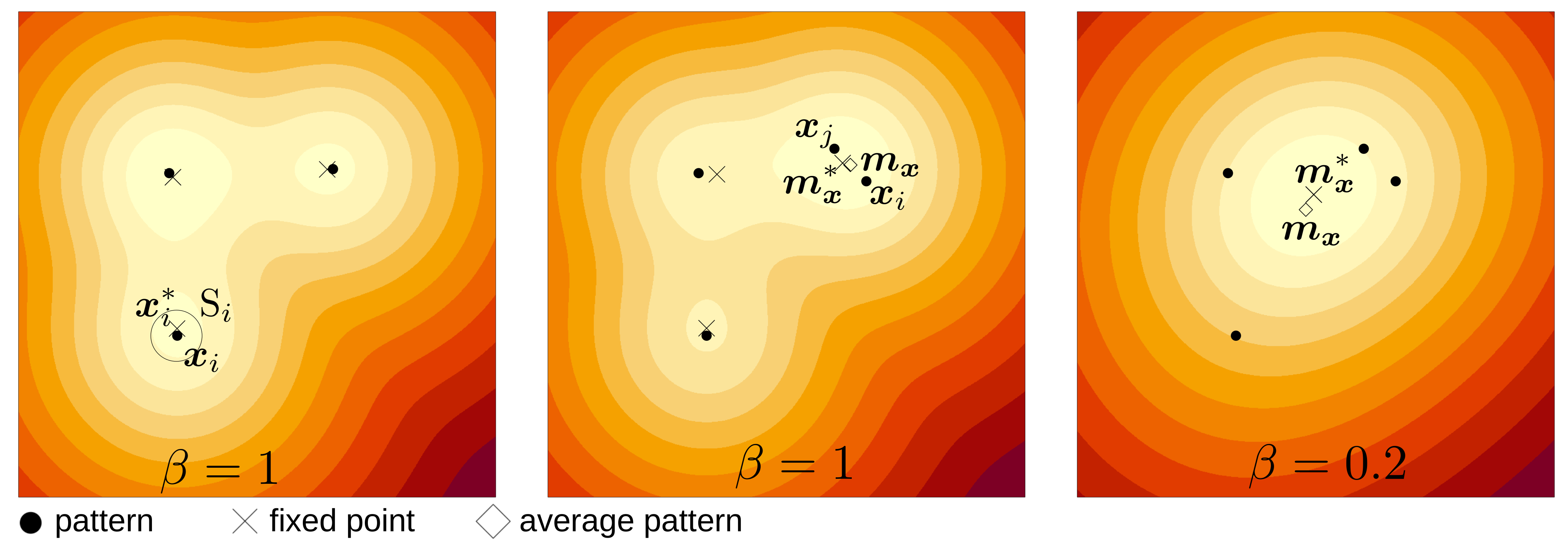
When all patterns form a sufficiently tight cluster, a contraction argument gives one fixed point near their mean. A separated subgroup can instead have a fixed point near its own mean. These global-average, cluster-average and individual-pattern regimes are established under the appendix’s quantitative conditions; absence of an individually isolated pattern alone is not a general uniqueness proof.
Hopfield update rule is attention of the transformer.
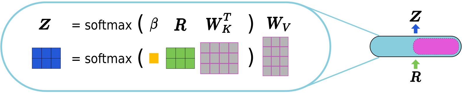
Project raw queries and keys into a common associative space and use β=1/√dₖ. A retrieval followed by a value projection gives softmax(QKᵀ/√dₖ)V. The derivation first factors V through the key representation; standard transformer attention allows a separate value map. Thus the attention weights and associative update coincide in the stated construction, while the fixed-memory energy proof applies directly in the associative space rather than automatically to arbitrary output/value dynamics.
Differentiability and useful single-step retrieval make the memory map suitable as a neural layer. Its proposed uses include set operations, attention, multiple-instance learning and access to reference data or learned prototypes; not every listed application is experimentally evaluated here.
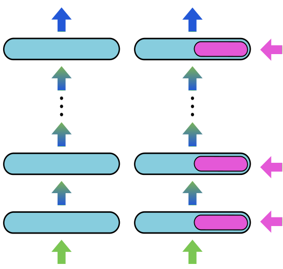
Figure 2: Left: A standard deep network with layers
() propagates
either a vector or a set of vectors from the input to the output.
Right: A deep network, where layers ()
are equipped with associative memories
via Hopfield layers ().
Types of neural networks.
The layer can operate in networks propagating one activation vector or a set of vectors. It supplies an associative memory at selected layers while retaining the surrounding feed-forward or recurrent computation.
Hopfield associates a query set with a stored set, both supplied by inputs or previous layers. HopfieldPooling uses learned static queries to summarize an input set into a fixed number of outputs; one query gives a bag representation for multiple-instance learning. HopfieldLayer keeps a fixed or learnable memory and accepts changing queries, enabling repeated access to training examples, prototypes or reference patterns. Memory inputs and target values can be separated so similarity-weighted retrieval predicts labels. These are architectural analogies to nearest-neighbor, prototype and support-vector methods, not a claim that every such algorithm is identical to one layer.
Figure 3: The layer Hopfield allows the association of two sets () and ().
It can be integrated into deep networks that propagate sets of vectors.
The Hopfield memory
is filled
with a set from either the input or previous layers.
The output is a set of vectors ().
Figure 4: The layer HopfieldPooling enables
pooling or summarization of sets,
which are obtained from the input or from previous layers.
The input ()
can be either a set or a sequence.
The query patterns of each layer are static and can be learned.
The output is a set of vectors (),
where the number of vectors equals the number of query patterns.
The layer HopfieldPooling can realize multiple instance learning.
Figure 5: The layer HopfieldLayer enables
multiple queries of the training set,
a reference set, prototype set, or a learned set (a learned matrix).
The queries for each layer are computed from the results of previous layers.
The input is a set of vectors (). The output is also a set of vectors (),
where the number of output vectors equals the number of input vectors.
The layer HopfieldLayer can realize
SVM models, -nearest neighbor, and LVQ.
Repeated updates refine retrieval without adding parameters. Temperature β controls concentration, associative dimension affects potential capacity, and normalization changes pattern norms and fixed-point geometry. These settings interact with learning rate and training dynamics; larger capacity does not by itself ensure useful learned memories.
4 Experiments
The experiments test the layer family across attention analysis, bag classification, small tabular data and molecular prediction. The appendix supplies the protocols and additional drug-design results.
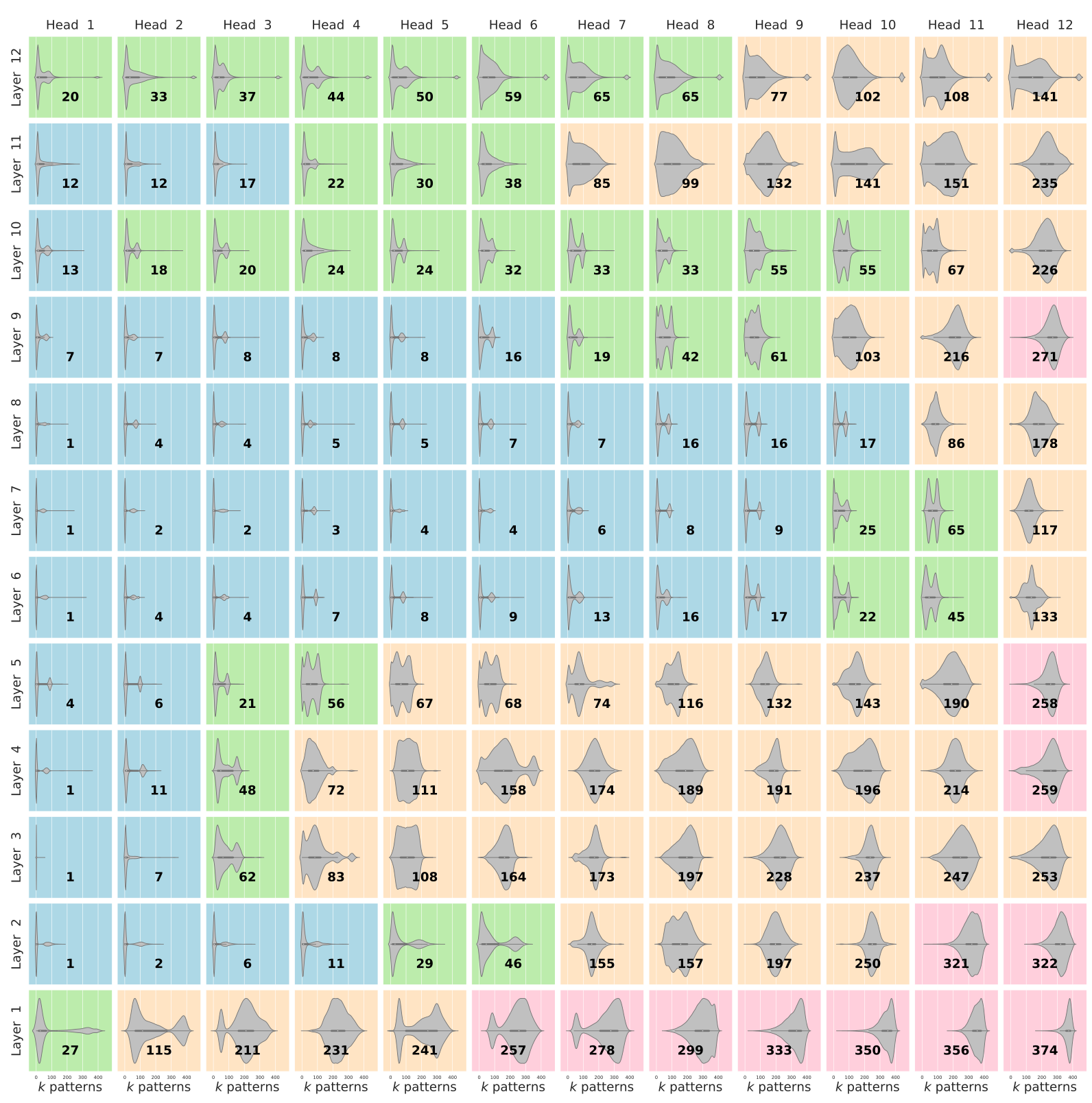
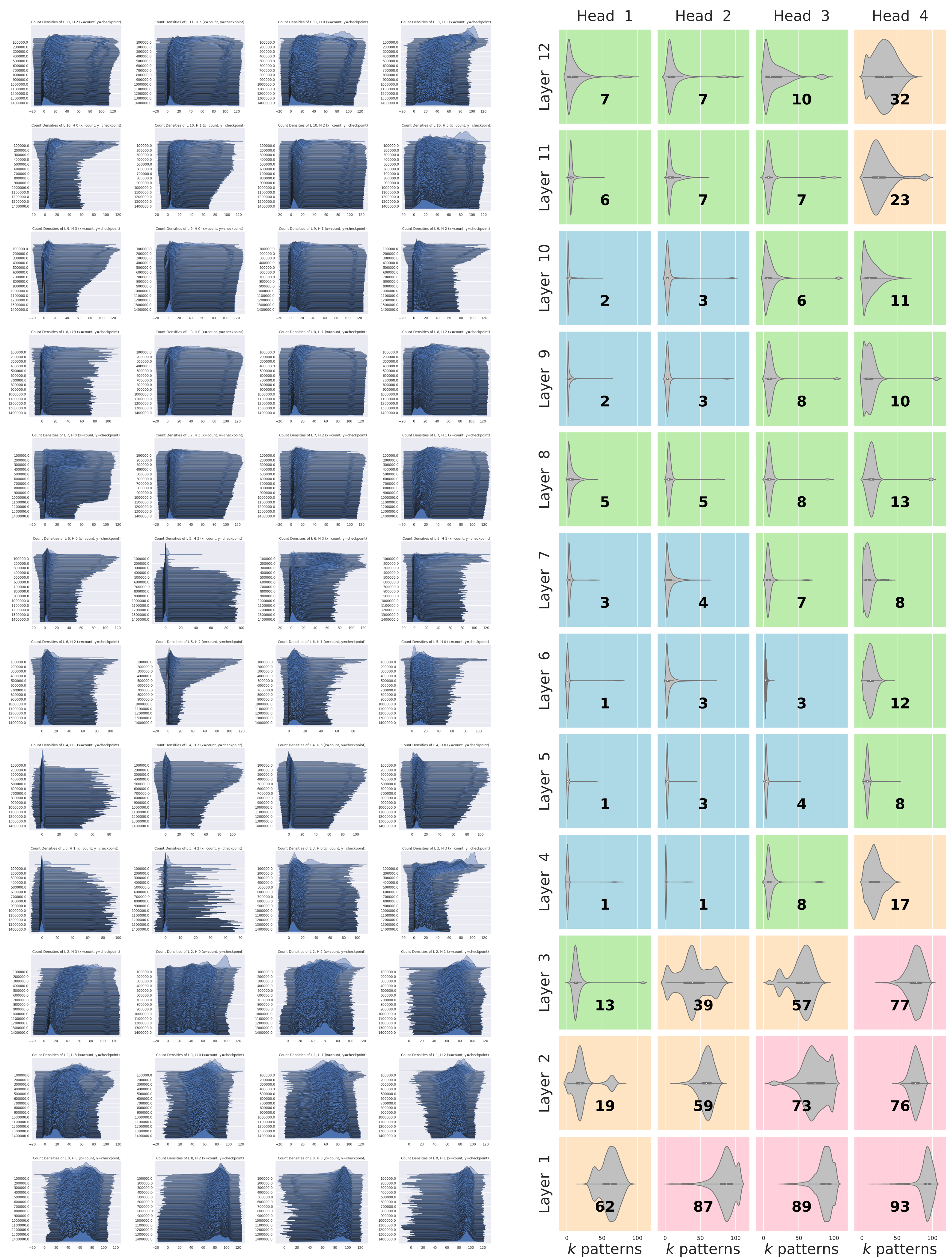
Sort attention weights and count the smallest k carrying 90% of their mass. Classify a head by the median k relative to sequence length: above N/2, (N/8,N/2], (N/32,N/8], or at most N/32. Lower BERT layers often average broadly, middle layers include both focused and broad heads, and higher layers favor intermediate concentration. This attention-concentration diagnostic is evidence about operating behavior; it is not a direct numerical verification that every head has converged to an energy minimum.
Multiple Instance Learning Datasets.
DeepRC pools receptor-sequence features from bags with roughly 300,000 instances. On the reported real repertoire dataset it achieves AUC .832±.022, versus .825±.022 for the MinMax-kernel SVM; overlapping variation cautions against interpreting the small gap as conclusive superiority on that dataset. Across the reported repertoire tasks its average is strongest. On the four smaller MIL benchmarks, HopfieldPooling leads Tiger, Elephant and UCSB but performs poorly on Fox (.6405 versus .738 for MILES). Table 1 uses previously published baseline results, choosing the higher reported AUC where two sources differ.
Table 1: Results for MIL datasets Tiger, Fox, Elephant, and
UCSB Breast Cancer in terms of AUC.
Results for all methods except the first are taken from either
a(Küçükaşcı &
Baydoğan, 2018) or b(Carbonneau et al., 2016),
depending on which reports the higher AUC.
On 75 UCI datasets with fewer than 1,000 samples, an SNN-based representation plus Hopfield retrieval has the best aggregate rank. The top three runner-up differences are not statistically significant by the reported Wilcoxon comparison; this is not dominance on every dataset. The appendix also tests training-set memories on HIV, BACE, BBBP and SIDER, reporting the best displayed results on BACE (.902±.023) and SIDER (.672±.019). These task-specific findings support useful associative layers without making the capacity theorem a generalization guarantee.
Table 2: Results on 75 small datasets of the UCI benchmarks
given as difference to average rank.
Acknowledgments
The authors acknowledge institutional, public and industrial support for the Linz research groups and IARAI.
Appendix A Appendix
The appendix develops continuous-memory theory, mathematical tools, prior binary-memory models, the attention correspondence, experiment details and the implementation interface. Its original formal statements and displayed derivations are retained alongside the condensed explanations.
A.1 Continuous State Modern Hopfield Networks (A New Concept)
This section establishes global energy behavior, local contraction regimes, storage/retrieval conditions and extensions for learned associations and changing memories.
A.1.1 Introduction
The theory proceeds from energy descent to local contraction, then uses separation to derive storage and retrieval bounds. Later subsections distinguish learning the association geometry from retrieval with a fixed memory, and discuss temporal weighting.
A.1.2 New Energy Function
The energy can also be written as a negative logarithm of weighted Gaussian similarities. A nearest-pattern comparison proves nonnegativity. For states in the convex hull of the memory vectors, Jensen’s inequality and norm bounds give both β⁻¹ ln N+M²/2 and 2M² upper bounds. Every retrieval enters this hull, but those upper bounds do not apply to an arbitrary unbounded initial query.
For in the simplex defined by the patterns,
the energy is upper bounded by:
Equations 17–18
(17)
(18)
Equations 19–27
(19)
(20)
(21)
(22)
(23)
(24)
(25)
(26)
(27)
A.1.3 New Update Rule
The update replaces the state by a softmax-weighted convex combination of stored patterns. This immediately confines subsequent states to their convex hull. Unlike the sign-based binary update, it remains continuous and differentiable.
Equations 28–30
(28)
(29)
(30)
A.1.4 Global Convergence of the Update Rule
Split the energy into a convex quadratic and concave negative log-sum-exp. Linearizing the concave term produces a tight quadratic upper bound whose unique minimizer is the retrieval update. The bound decreases strictly whenever the state changes. Compactness and the cited convergence results imply stationary limit points, vanishing step sizes and either convergence or a connected compact stationary limit set. A finite stationary set at the limiting energy ensures convergence to one point. These results establish energy descent, not global optimality or a uniform convergence rate.
For the iteration Eq. (55)
we have
as , for some stationary point .
Furthermore and
either converges
or, in the other case, the set of limit points of
is a connected and compact subset of , where
and is the set of stationary points of the iteration Eq. (55).
If is finite, then any sequence
generated by the iteration Eq. (55)
converges to some .
Equation 56
(56)
A.1.5 Local Convergence of the Update Rule: Fixed Point Iteration
Local convergence uses Banach’s fixed-point theorem: first find a closed invariant neighborhood, then bound the retrieval Jacobian below one throughout it. A small Jacobian also yields a fast rate.
A.1.5.1 General Bound on the Jacobian of the Iteration.
The symmetric Jacobian is βX(diag(p)−ppᵀ)Xᵀ, equivalently β times the attention-weighted covariance of stored patterns. Its norm is bounded using pattern norms and max pᵢ(1−pᵢ); concentration near one pattern makes it small. Separation Δᵢ measures the self-dot-product advantage over competing memories. For equal-norm patterns it equals half the nearest squared Euclidean distance. Figure A.1 illustrates the three regimes, while the following lemmas give their sufficient conditions.
Equations 57–59
(57)
(58)
(59)
Figure A.1: The three cases of fixed points.
a) Stored patterns (fixed point is single pattern):
patterns are stored if they are well separated.
Each pattern has a single fixed point close to it.
In the sphere , pattern is the only pattern and the only fixed point.
b) Metastable state (fixed point is average of similar patterns):
and are similar to each other and not
well separated. The fixed point is a metastable state
that is close to the mean of the similar patterns.
c) Global fixed point (fixed point is average of all patterns):
no pattern is well separated from the others.
A single global fixed point exists that is close to
the arithmetic mean of all patterns.
For patterns ,
, , and
, the spectral norm of the Jacobian
of the fixed point iteration
is bounded:
Equation 60
(60)
If , then for the spectral norm of
the Jacobian holds
Equation 61
(61)
Equations 62–69
(62)
(63)
(64)
(65)
(66)
(67)
(68)
(69)
Definition 2(Separation of Patterns).
We define , i.e. the separation of pattern from data as:
Equation 70
(70)
The pattern is separated from the other data if .
Using the parallelogram identity, can also be expressed as
Equation 71
(71)
For we have .
Analog we say for a query and data ,
that is least separated from while
being separated from other with if
Equations 72–73
(72)
(73)
A.1.5.2 One Stable State: Fixed Point Near the Mean of the Patterns.
Let m be the pattern mean and r=maxᵢ‖xᵢ−m‖. The covariance bound gives ‖J‖₂≤βr², so βr²<1 makes retrieval contractive on its invariant convex hull and yields a unique fixed point. If the data are centered, zero is exactly a fixed point with uniform weights. Further estimates relate near-uniform attention to spread, centering and the Gram matrix. Uniform-looking weights alone do not imply small covariance for arbitrarily large pattern norms. The source’s phrase “in each compact set” also needs the map-to-itself condition required by Banach’s theorem.
The following bound on the norm of the
Jacobian of the fixed point iteration holds independent of or
the query .
Equation 82
(82)
For there exists
a unique fixed point (global fixed point) of iteration in each compact set.
Equations 83–129
(83)
(84)
(85)
(86)
(87)
(88)
(89)
(90)
(91)
(92)
(93)
(94)
(95)
(96)
(97)
(98)
(99)
(100)
(101)
(102)
(103)
(104)
(105)
(106)
(107)
(108)
(109)
(110)
(111)
(112)
(113)
(114)
(115)
(116)
(117)
(118)
(119)
(120)
(121)
(122)
(123)
(124)
(125)
s.t.
(126)
(127)
(128)
(129)
A.1.5.3 Many Stable States: Fixed Points Near Stored Patterns.
For a query whose preferred pattern has a positive score margin, total competing attention is at most (N−1)e^(−βmargin). This bounds the updated state’s distance from that pattern. Lemmas A5–A7 use a ball of radius 1/(βNM), sufficient pattern separation, invariance and a Jacobian bound to obtain a unique attracting fixed point. The state generally converges near the stored vector, not exactly to it. A mean-value bound then makes the one-step error small when the separation overwhelms the competing-pattern count and query distance.
Lemma A4.
For a query and data ,
there exists a that is least separated from while
being separated from other with :
A.1.5.4 Metastable States: Fixed Points Near Mean of Similar Patterns.
For a cluster of l similar patterns, split attention into within-cluster mass 1−γ and leakage γ. The Jacobian bound combines within-cluster spread with a term of order βγM² from outside patterns. Lemmas A9–A12 require a compact neighborhood around the cluster mean, sufficient separation from the remaining memories and a sufficiently small cluster radius. These ensure invariance and contraction toward a cluster fixed point. The final bounds show why a tightly packed, well-isolated cluster can converge rapidly even when no individual member is separately retrieved.
Equations 187–200
(187)
(188)
(189)
(190)
(191)
(192)
(193)
(194)
(195)
(196)
(197)
(198)
(199)
(200)
Lemma A8.
With the definitions in Eq. (193)
to Eq. (200),
the following bounds on the norm of the
Jacobian of the fixed point iteration hold.
The -bound for is
A.1.6 Properties of Fixed Points Near Stored Pattern
Capacity and retrieval quality trade off through separation. Packing more patterns closer together can reduce attraction margins, slow convergence and increase error. Storage here requires disjoint basins with unique attracting fixed points; it is more specific than merely counting stationary points.
A.1.6.1 Exponentially Many Patterns can be Stored.
The master inequality relates minimum separation to N, β and the largest norm M. For equal-radius patterns, separation becomes M²(1−cos α_min), allowing spherical-packing arguments. The placed-pattern claims in Theorems A3–A4 use Equation 315’s angular-coordinate counting rule as if it guaranteed pairwise angular spacing. It does not in general: A3’s d=4 example would require 64 vectors separated by at least π/2 in four dimensions, whereas at most eight can have pairwise nonpositive inner products. Those displayed claims and their proof remain unchanged, but the construction is not established as written.
The random-pattern result follows a separate route: a lower-tail bound on the minimum angle, estimates of its dimension-dependent constant, and a cosine bound. Theorem A5 solves the sufficient inequality using the principal Lambert W branch, giving a capacity lower bound √p·c^((d−1)/4) with failure probability p and radius K√(d−1), subject to its stated admissibility conditions. The cited examples use β=1,p=.001 and either K=3,d=20 or K=1,d=75. Corollary A1 replaces Lambert W with simpler bounds; Theorem A6 and Corollary A2 solve for dimension using the appropriate branch. Theorem A7 instead substitutes an expected minimum separation into the criterion; this is not the same as a high-probability guarantee that every random memory is retrievable.
Equations 297–299
(297)
(298)
(299)
Definition 5(Pattern Stored and Retrieved).
We assume that around every pattern a sphere is given.
We say is stored if there is a single fixed point to
which all points converge,
and for .
We say is retrieved for a given if
iteration (update rule) Eq. (92) gives
a point that is at least
-close to the single fixed point .
The retrieval error is .
We assume and patterns on the sphere with radius .
If and the dimension
of the space is or if
and the dimension
of the space is ,
then
the number of patterns that can be stored
(fixed point with attraction basin near pattern) is
at least
We assume and patterns on the sphere with radius .
If and the dimension
of the space is or if
and the dimension
of the space is ,
then
the number of patterns that can be stored
(fixed point with attraction basin near pattern) is
at least
We have the following lower bound on the expectation of :
Equation 383
(383)
The bound is valid for all and .
Lemma A17.
The following estimate holds for :
Equation 384
(384)
Equations 385–386
(385)
(386)
Theorem A7(Storage Capacity (expected separation): Random Patterns).
We assume patterns on the sphere with radius
that are randomly chosen.
Then for all values for which
Equation 387
(387)
holds,
the number of stored patterns for the expected minimal separation is at least
Equation 388
(388)
The inequality Eq. (387) is e.g. fulfilled with , , and .
Equations 389–392
(389)
(390)
(391)
(392)
A.1.6.2 Retrieval of Patterns with One Update and Small Retrieval Error.
Theorems A8–A9 distinguish error to the local fixed point from error to the original stored vector. Both decay exponentially in the separation margin after accounting for the query/fixed-point distances, β, M and competing-pattern count. The Gaussian-pair calculation illustrates how typical separation grows with dimension; it does not by itself bound the minimum over exponentially many competitors. One-step retrieval is therefore a local, margin-dependent statement rather than convergence from every query.
Theorem A8(Pattern Retrieval with One Update).
With query , after one update the distance of the new point
to the fixed point is exponentially small in the separation .
The precise bounds using the Jacobian and its value in the mean value
theorem are:
Equations 393–394
(393)
(394)
For given and
sufficient large , we have ,
that is, retrieval with one update.
Equations 395–400
(395)
(396)
(397)
(398)
(399)
(400)
Theorem A9(Exponentially Small Retrieval Error).
The retrieval error of pattern
is bounded by
Equation 401
(401)
and for
together with
by
Equation 402
(402)
Equations 403–405
(403)
(404)
(405)
A.1.7 Learning Associations
Association can use raw patterns, one learned bilinear map, or separate query/key projections into a shared lower-dimensional space. The following derivatives explain how these retrieval operations participate in backpropagation.
A.1.7.1 Association of Raw Patterns – No Mapping in an Associative Space.
For raw queries and stored patterns, differentiating the update gives the familiar covariance Jacobian with respect to the query. The memory gradient additionally contains a direct weighted-output term because changing a stored pattern changes both its score and its retrieved value.
Equations 406–409
(406)
(407)
(408)
(409)
A.1.7.2 Learning an Association Matrix – Only One Set is Mapped in an Associative Space.
One map can transform keys into query space, queries into key space, or define the bilinear association directly. The full recurrent update includes the transformed memory values; the simplified final-step version can absorb an outer map into the value projection. The displayed gradients distinguish these cases, adding the direct output contribution when differentiating the full map. Repeated retrieval must remain in the associative space.
Equations 410–420
(410)
(411)
(412)
(413)
(414)
(415)
(416)
(417)
(418)
(419)
(420)
A.1.7.3 Learning Two Association Mappings – Both Sets are Mapped in an Associative Space.
Separate key and query maps factor the association matrix through dimension dₖ. The appendix derives gradients for each map, including the additional direct term for keys in the full update. A simplified output may live in raw-key space, so applying it repeatedly without the stated mapping would change the dynamics. These formulas train the geometry; the earlier convergence results analyze retrieval after that geometry is fixed.
Equations 421–437
(421)
(422)
(423)
(424)
(425)
(426)
(427)
(428)
(429)
(430)
(431)
(432)
(433)
(434)
(435)
(436)
(437)
A.1.8 Infinite Many Patterns and Forgetting Patterns
Temporal use extends the current memory as observations arrive and can reduce the influence of older entries. These mechanisms alter the active memory or attention scores rather than proving unlimited storage with fixed computational cost.
A.1.8.1 Infinite Many Patterns.
At time t, retrieve only from the observed prefix Xₜ. Causal masking expresses the same restriction in attention notation. The “infinite” construction is a formal stream interpretation: each actual finite-time update uses the available prefix, and storage/computation can grow with t.
Equations 438–448
(438)
(439)
(440)
(441)
(442)
(443)
(444)
(445)
(446)
(447)
(448)
A.1.8.2 Forgetting Patterns.
Subtract an age-dependent term from an old pattern’s logit to obtain exponentially decreasing temporal weight. The printed energy451 includes βγ(t−i), while452 uses γ(t−i), and updates453–454 omit that age term. These original formulas remain unchanged. An implementation must choose and consistently apply its intended time penalty in both energy and softmax; the printed sequence does not define that choice consistently.
Equations 449–454
(449)
(450)
(451)
(452)
(453)
(454)
A.1.9 Number of Spurious States
A monotone transformation of the energy relates its minima to modes of a weighted isotropic Gaussian mixture. Such a mixture can have more modes than components, so a memory may possess additional stable states beyond the N intended pattern states. High storage capacity does not imply that all spurious states disappear.
Equations 455–458
(455)
(456)
(457)
(458)
A.2 Properties of Softmax, Log-Sum-Exponential, Legendre Transform, Lambert W Function
Softmax is the gradient of log-sum-exp. Its Jacobian β(diag(p)−ppᵀ) is positive semidefinite, annihilates the all-ones vector and has spectral norm at most β/2; concentrated probabilities give tighter local bounds. These facts supply monotonicity, Lipschitz and cocoercivity statements. The section also develops convex-conjugate rules, the entropy/log-sum-exp duality, Lambert W identities used in capacity calculations, and an integral-Jacobian mean-value formula.
The basic entropy duality is standard, but Lemma A29’s formula/domain for log-sum-exp composed with a rectangular matrix is not generally valid as written. For X=[0,1], XXᵀ is nonsingular and log(1+e^ξ) has a finite conjugate on [0,1], while the proposed pseudoinverse-based simplex constraint does not recover that domain. The original lemma and proof remain for inspection; the earlier direct covariance and energy-descent arguments do not require this domain formula.
with .
The is the maximum of on
the -dimensional
simplex with :
Equation 466
(466)
The softmax is the argument
of the maximum of on
the -dimensional
simplex with :
Equation 467
(467)
Lemma A20.
The Jacobian of the softmax is
Equation 468
(468)
which gives the elements
Equation 469
(469)
Lemma A21.
The Jacobian of the softmax function
has a zero eigenvalue with eigenvector .
Equation 470
(470)
Lemma A22.
The Jacobian of the softmax
is symmetric and positive semi-definite.
Equation 471
(471)
Lemma A23.
The softmax is monotone for , that is,
Equation 472
(472)
Equations 473–475
(473)
(474)
(475)
Lemma A24.
For a softmax with
, the spectral norm of
the Jacobian of the softmax is bounded:
Equations 476–478
(476)
(477)
(478)
In particular everywhere holds
Equation 479
(479)
If , then for the spectral norm of
the Jacobian holds
Equation 480
(480)
Equations 481–487
(481)
(482)
(483)
(484)
(485)
(486)
(487)
Lemma A25.
The softmax function
is -Lipschitz.
The softmax function
is -Lipschitz
in a convex environment for which
.
For ,
the softmax function
is -Lipschitz.
For , the softmax
is contractive in on which is defined.
Equations 488–492
(488)
(489)
(490)
(491)
(492)
Lemma A26.
For ,
softmax function
is -cocoercive in , that is,
Equation 493
(493)
In particular
the softmax function
is -cocoercive everywhere.
With ,
the softmax function
is -cocoercive in .
The Lambert function has an upper branch for and a lower
branch for .
We use if a formula holds for both branches.
We have
Equation 516
(516)
Lemma A30.
Identities for the Lambert function are
Equations 517–529
(517)
(518)
(519)
(520)
(521)
(522)
(523)
(524)
(525)
(526)
(527)
(528)
(529)
Lemma A31.
Equations 530–538
(530)
(531)
(532)
(533)
(534)
(535)
(536)
(537)
(538)
where the Omega constant is
Equation 539
(539)
Lemma A32(Mean Value Theorem).
Let be open, continuously differentiable, and
as well as vectors such that the line segment
for is in . Then the following holds:
Equation 540
(540)
where is the Jacobian of and the integral of the matrix is component-wise.
Equations 541–542
(541)
(542)
A.3 Modern Hopfield Networks: Binary States (Krotov and Hopfield)
The appendix relates the proposed continuous network to earlier binary modern Hopfield networks. Their interaction functions, coordinatewise dynamics and probabilistic capacity results are distinct from the continuous update analyzed above.
The background separates external memory architectures from the development of high-capacity binary associative memories.
A.3.1.1 Additional Memory and Attention for Neural Networks.
Neural Turing machines explicitly read and write an external memory; memory networks provide input, generalization, output and response components. End-to-end memory networks replace a discrete memory selection with differentiable softmax. The review traces connections to recurrent associative memories, key/value attention, transformers and BERT. Similar mechanisms do not imply identical energies, learning rules or retrieval guarantees.
Capacity depends on the update rule, pattern distribution, required stability and allowable error. The appendix contrasts classical binary capacities with polynomial interactions and exponential interactions. Exponentially many energy minima are not the same as exponentially many reliably retrievable intended memories. The reported earlier exponential-capacity result uses random binary patterns and a probability statement tied to the permitted corruption radius.
A.3.2 Energy and Update Rule for Binary Modern Hopfield Networks
For binary states, an interaction function is applied to each pattern–state inner product and summed into the energy. A coordinate update compares the energies of setting that coordinate to +1 or −1. Theorem A10 quotes the exponential-interaction result: random-pattern storage rate must stay below a corruption-dependent large-deviation threshold, and one update of each component recovers the target with probability tending to one as dimension grows. The proof is delegated to Demircigil et al. The subsequent mean-value argument expresses the coordinate decision through a softmax-weighted pattern sum, motivating the continuous construction without equating the two dynamics.
Equations 543–545
(543)
(544)
(545)
Theorem A10(Storage Capacity for Binary Modern Hopfield Nets (Demircigil et al. 2017)).
Consider the generalized Hopfield model with the dynamics
described in Eq. (545) and
interaction function given by .
For a fixed
let and let
be patterns chosen uniformly at random from .
Moreover fix .
For any and any taken uniformly at random
from the Hamming sphere with radius centered in ,
, where is assumed to be an integer,
it holds that
Equation
if is chosen in dependence of such that
Equation
with
Equation
Equations 546–547
(546)
(547)
A.4 Hopfield Update Rule is Attention of The Transformer
Map queries and keys into the same associative space, apply one Hopfield update with β=1/√dₖ, and project the result into value space. Equation548 becomes the usual scaled dot-product attention formula. Here the values factor through the projected keys as K Wᵥ; the correspondence identifies this retrieval computation, not every residual, normalization or feedforward component of a transformer. Repeated energy-descent guarantees concern fixed memories and the specified associative state update.
Equation 548
(548)
Figure A.2: We generalized
the energy
of binary modern Hopfield networks for allowing continuous states
while keeping fast convergence and
storage capacity properties.
We defined for the new energy also a new update
rule that minimizes the energy.
The new update rule is the attention mechanism of the transformer.
Formulae are modified to express as row vector as for transformers.
""-sign means "keeps the properties".
A.5 Experiments
Additional experiments describe attention-head behavior, massive and conventional multiple instance learning, small tabular datasets, and molecular classification. Their datasets, validation procedures and metrics differ.
A.5.1 Experiment 1: Attention in Transformers described by Hopfield dynamics
The attention experiments classify heads by how many patterns account for90% of their probability mass, track that statistic through training, and test input-independent Gaussian averaging replacements.
A.5.1.1 Analysis of operating modes of the heads of a pre-trained BERT model.
For pretrained bert-base-cased, Figure A.3 displays a distribution of the smallest count k accumulating90% of attention mass for every head. Heads are sorted within each layer, so columns do not track a fixed head identity across layers. Large-averaging heads are common in lower layers; small metastable states often appear in middle layers; medium states occur toward the top. These are descriptive classes based on attention concentration, not a direct measurement proving convergence to a unique energy minimum.
Figure A.3: Analysis of operating modes of the heads of a pre-trained BERT model.
For each head in each layer, the distribution of the minimal number
of patterns required to sum up the values to is displayed as a violin plot in a panel.
indicates the size of a metastable state.
The bold number in the center of each panel gives the median of the distribution.
The heads in each layer are sorted according to .
Attention heads belong to the class they mainly operate in.
Class (IV) in blue:
Small metastable state or fixed point close to a single pattern, which
is abundant in the middle layers (6, 7, and 8).
Class (II) in orange: Large metastable state, which is
prominent in middle layers (3, 4, and 5).
Class (I) in red: Very large metastable state or global fixed point,
which is predominant in the first layer.
These heads can potentially be replaced by averaging operations.
Class (III) in green: Medium metastable state,
which is frequently observed in higher layers.
We hypothesize that these heads are used to collect information required to
perform the respective task.
These heads should be the main target to improve transformer and BERT models.
A.5.1.2 Experimental Setup.
The training study uses a reduced BERT-small model:12layers,4heads, hidden size256, embedding size128, sequence length128 and batch size128. It trains1.45million updates, reported as roughly four days on one V100. The data approximate the original Wikipedia/BookCorpus protocol, but use an uncased BookCorpus snapshot because of access restrictions. These details limit direct comparisons with full BERT training.
A.5.1.3 Hopfield Operating Classes of Transformer and BERT Models.
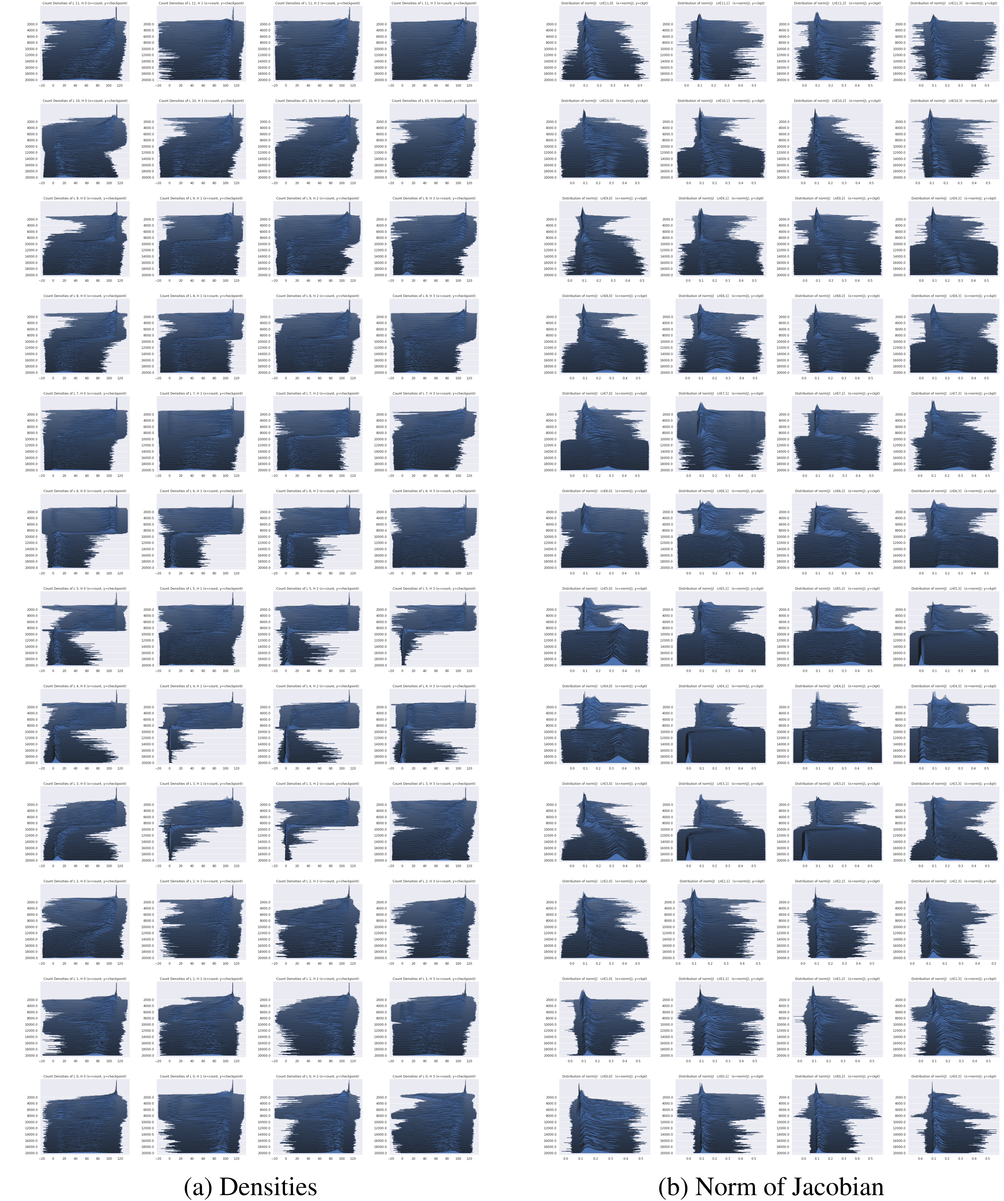
Figure A.4 tracks the distribution of90%-mass counts during BERT-small training and groups the final counts into four classes. Thresholds are divided by four to account for the reduction from512 to128tokens. Some heads commit early to small metastable-state behavior. This rescaled classification is a heuristic description of attention concentration.
A.5.1.4 Learning Dynamics of Transformer and BERT Models.
During the first20,000steps, several middle-layer heads change toward concentrated attention around9,000–10,000steps, near a second loss decrease. Figure A.5 also tracks the Frobenius norm of the softmax Jacobian. The reported later stability of these heads’ attention does not on its own prove that the mode transition caused the loss change or that every parameter gradient vanishes: the Jacobian is one factor in the full derivative.
Figure A.4: Left: Ridge plots of the distribution of counts over time for BERT-small Right: Violin plot of counts after steps, divided into the four classes from the main paper. The thresholds were adapted to the shorter sequence length.Figure A.5: (a): change of count density during training is depicted for the first steps.
(b): the corresponding distribution of the Frobenius norm of the Jacobian of the function
is depicted.
The gradients with respect to the weights are determined by the Jacobian defined in Eq. (59)
as can be seen in Eq. (418), Eq. (429), and Eq. (435).
A.5.1.5 Attention Heads Replaced by Gaussian Averaging Layers.
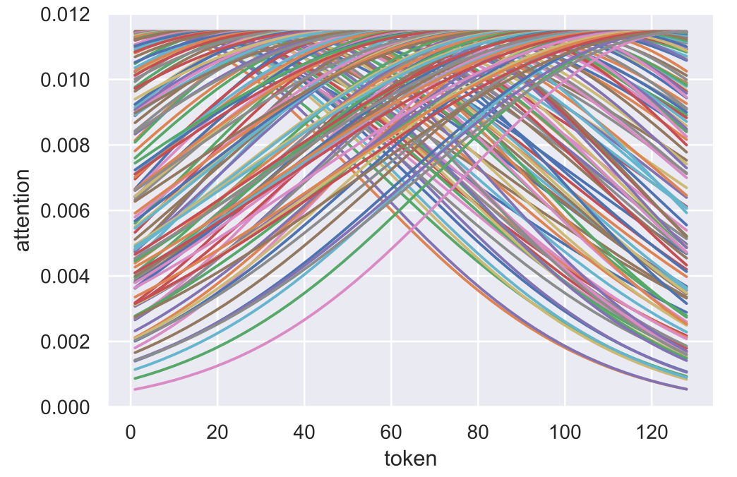
Gaussian averaging heads replace query-dependent scores with normalized discrete Gaussian kernels over token positions. Each position has a learned location and scale. Initialization samples locations in[−1,1] and scales in[.75,1.25], or centers each kernel at its corresponding support point; Figure A.6 shows the latter option. This uses2N location/scale parameters per head instead of the2dₖdᵧ query/key projection parameters being compared. The printed BERT-base arithmetic gives95.5×, although the displayed dimensions yield96×. This count excludes other attention components and trades input-dependent expressiveness for a smaller positional mechanism; it is not a whole-model parameter or runtime ratio.
Equations
Figure A.6: Attentions of a Gaussian averaging head at initialization for sequence length . Every line depicts one Gaussian kernel. Here, the location parameters are initialized with the value of the supporting points .
Multiple instance learning predicts a bag-level label from many instances. The experiments distinguish large immune-sequence repertoires from smaller image and histopathology bags.
A.5.2.1 Immune Repertoire Classification.
DeepRC maps immune amino-acid sequences through a position-aware one-dimensional convolutional network and uses learned static queries to pool class-indicative instances. The tests include simulated, LSTM-generated and real repertoires with implanted motifs, plus a real CMV-status dataset; several categories contain about300,000sequences per repertoire. The complete table retains every motif frequency and comparison. On real CMV, DeepRC reports AUC .832±.022 versus .825±.022 for the MinMax SVM, with errors across five folds. The difference is small relative to those deviations and is not presented here as a significance test. Implanted-signal results and biological generalization answer different questions; the capacity theorem alone does not guarantee either empirical result.
Table A.1: Results immune repertoire classification across all datasets. Results are given in terms of AUC of the competing methods on all datasets. The reported errors are standard deviations across cross-validation (CV) folds (except for the column “Simulated”).
Real-world CMV: Average performance over
CV folds on the cytomegalovirus (CMV) datasetEmerson et al. (2017).
Real-world data with implanted signals: Average performance over
CV folds for each
of the four datasets. A signal
was implanted with a frequency (=wittness rate) of
or . Either a single motif (“OM”)
or multiple motifs (“MM”) were implanted.
LSTM-generated data: Average performance over
CV folds for each
of the datasets. In each dataset, a signal
was implanted with a frequency of ,
, , , and , respectively.
Simulated: Here we report the mean over 18 simulated datasets with implanted signals and varying difficulties. The error reported is the standard deviation of the AUC values across the 18 datasets.
Elephant, Fox and Tiger each have200image bags, represented by region descriptors; UCSB has58histopathology bags and2,002patch instances. Embedded instances enter HopfieldPooling with a trainable static query, followed by a classifier. A manual validation-set search varies widths, head counts, associative dimensions, β and regularization. Train160epochs with AdamW and exponential learning-rate decay; report average AUC from five repetitions of nested ten-fold cross-validation. Bag dropout addresses the severe small-data overfitting risk. Table A.2 retains the full search space.
parameter
values
learning rates
,
learning rate decay (γ)
embedding layers
layer widths
number of heads
head dimensions
scaling factors
hidden dimensions
bag dropout
Table A.2: Hyperparameter search-space of a manual hyperparameter selection on the respective validation sets of the Elephant, Fox, Tiger and UCSB breast cancer datasets.
A.5.3 Experiment 3: Classification on Small UCI Benchmark Datasets
A learned associative memory supplies prototypes for classification on75small UCI datasets. The protocol uses held-out validation and test sets, rather than the multiple-instance cross-validation scheme.
A.5.3.1 Motivation.
An optional self-normalizing embedding feeds a Hopfield layer with learned stored patterns; its retrieved output feeds the classifier. The motivation is to learn class-indicative prototypes for datasets with fewer than1,000samples, where standard neural networks often struggle. The number of patterns and associative dimension are hyperparameters rather than fixed theoretical optima.
A.5.3.2 Methods compared.
The comparison spans17families, including SVMs, forests, boosting, regression and discriminant methods, bagging, nearest neighbors, trees, ensembles, Bayesian methods and multiple neural-network variants. These categories encompass the25methods used in the final rank comparison; a family label is not a separate uniform implementation.
A.5.3.3 Experimental design and implementation details.
For each dataset, search the architecture and hyperparameters in Table A.3. Train up to100epochs with cross entropy, batch size4, and SGD without momentum, weight decay or dropout. Early stopping selects the model using validation accuracy averaged over16consecutive epochs; the selected model is evaluated on a separate test set. Embedding depth is0/1/7, width32/128/1024, and the number of stored patterns is one or eight times the class count. Validation selection and historical baseline scores should be considered when interpreting aggregate ranks.
parameter
values
learning rates
embedding layers
hidden units
heads
# stored patterns
Table A.3: Hyperparameter search-space for grid-search on small UCI benchmark datasets.
All models were trained for epochs using stochastic gradient descent
with early stopping based on the validation set accuracy and
a minibatch size of samples.
The number of stored patterns is depending on the number of target classes of the individual tasks.
A.5.3.4 Results.
Rank each of25methods by test accuracy within each dataset, then average those ranks across the75datasets. The baseline scores come from the cited earlier study. A rank difference is not an average percentage-point accuracy gain, and this aggregate does not establish superiority for every dataset.
A.5.4 Experiment 4: Drug Design Benchmark Datasets
The molecular experiments retrieve information from a reference set of training compounds and labels. This is a different use of the layer from a learned static prototype matrix.
A.5.4.1 Experimental design and implementation details.
Evaluate HIV, BACE, BBBP and SIDER from MoleculeNet. The training inputs act as stored keys, labels as retrieved values, and the current compound as query. Separate validation sets select β, head count, normalization, bias, dropout and other choices in Table A.4. The source describes selecting the highest-validation-AUC model on five random splits; the result table describes50random splits, so that discrepancy is retained rather than silently resolved. Applicable learned models train four epochs with Adam and batch size1. Test labels must remain outside the stored training reference set.
parameter
values
beta
learning rates
heads
dropout
state-pattern bias
association-activation
{None, LeakyReLU }
state- and stored-pattern static
{False, True}
normalize state- and stored-pattern
{False, True}
normalize association projection
{False, True}
learnable stored-pattern
{False, True}
Table A.4: Hyperparameter search-space for grid-search on HIV, BACE, BBBP and SIDER.
All models were trained if applicable for epochs using
Adam and a batch size of sample.
A.5.4.2 Results.
Table A.5 compares against SVM, XGBoost, forests, dense neural networks and several graph models, with historical baseline results taken from Jiang et al. The Hopfield layer reports ROC-AUC .902±.023 on BACE and .672±.019 on SIDER, the best table entries for those datasets. It does not win every dataset. The comparison combines reported baselines with the stated validation protocol, and its split-count discrepancy prevents treating every cell as a fully controlled rerun.
Table A.5: Results on drug design benchmark datasets. Predictive performance (ROCAUC) on test set as reported by Jiang et al. (2020) for 50 random splits
The authors provide a PyTorch implementation at ml-jku/hopfield-layers. The appendix explains the source-version interface and its relation to the mathematical update; it is not a claim that every present-day release retains exactly the same API.
A.6.1 Introduction
Hopfield layers can associate sets, pool a variable-size bag, or retrieve from prototypes, training examples or a reference memory. The appendix relates the raw queries R and stored patterns Y to associative queries Q and keys K, then projects retrieved states into output values. Permutation-invariant pooling requires an appropriate query/output arrangement; sequence-order tasks may additionally need positional information.
A.6.2 Functionality
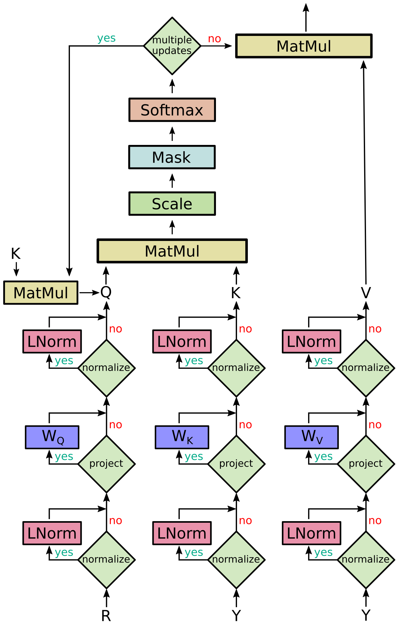
The interface exposes six main controls. Query/key projections associate two possibly different input sets. Multiple updates iterate in associative space before the final value projection, with a maximum count or state-change tolerance. β controls concentration together with pattern geometry and affects gradients. Associative dimension affects separation and representational capacity, with larger dimensions also increasing computation. Static patterns are independent of the current input but can be learned through backpropagation. Optional normalization changes pattern norms and centers, which influence averaging and metastable behavior. Figure A.7 preserves the complete flow, including the separate key and value inputs. Theorems for fixed patterns give intuition for these choices but do not prescribe a universally optimal β, dimension or normalization during training.
Equations 549–555
(549)
(550)
(551)
(552)
(553)
(554)
(555)
Figure A.7:
A flowchart of the Hopfield layer.
First, the raw state (query) patterns
and the raw stored (key) patterns
are optionally normalized (with layer normalization),
projected and optionally normalized (with layer normalization) again.
The default setting is a layer normalization of the input
patterns, and no layer normalization of the projected patterns.
The raw stored patterns can in principle be also two different input tensors.
Optionally, multiple updates take place in the
projected space of and .
This update rule is obtained e.g. from the full update
Eq. (423) or the simplified update
Eq. (424)
in the appendix.
A.6.3 Usage
The module can implement pooling, set association and attention, while encoder/decoder wrappers recover the corresponding PyTorch transformer-style behavior with the extra functionalities disabled. It can also replace recurrent components in some designs, but matching the information flow, sequence order, masks, tensor shapes and recurrent semantics requires an architecture-specific choice. A substitution is an interface capability rather than a guarantee of identical learned behavior.
119 references
Abu-Mostafa & StJacques (1985)
Y. Abu-Mostafa and J.-M. StJacques.
Information capacity of the Hopfield model.
IEEE Transactions on Information Theory, 31, 1985.
doi: 10.1109/tit.1985.1057069.
Agrawal et al. (1993)
R. Agrawal, T. Imieliundefinedski, and A. Swami.
Mining association rules between sets of items in large databases.
SIGMOD Rec., 22(2):207–216, 1993.
doi: 10.1145/170036.170072.
Akbar et al. (2019)
R. Akbar, P. A. Robert, M. Pavlović, J. R. Jeliazkov, I. Snapkov,
A. Slabodkin, C. R. Weber, L. Scheffer, E. Miho, I. H. Haff, et al.
A compact vocabulary of paratope-epitope interactions enables
predictability of antibody-antigen binding.
bioRxiv, 2019.
Alzahrani & Salem (2018)
F. Alzahrani and A. Salem.
Sharp bounds for the lambert function.
Integral Transforms and Special Functions, 29(12):971–978, 2018.
Andrews et al. (2003)
S. Andrews, I. Tsochantaridis, and T. Hofmann.
Support vector machines for multiple-instance learning.
In S. Becker, S. Thrun, and K. Obermayer (eds.), Advances in
Neural Information Processing Systems 15, pp. 577–584. MIT Press, 2003.
Ba et al. (2016a)
J. Ba, G. E. Hinton, V. Mnih, J. Z. Leibo, and C. Ionescu.
Using fast weights to attend to the recent past.
In D. D. Lee, M. Sugiyama, U. V. Luxburg, I. Guyon, and R. Garnett
(eds.), Advances in Neural Information Processing Systems 29, pp. 4331–4339. Curran Associates, Inc., 2016a.
Ba et al. (2016b)
J. Ba, G. E. Hinton, V. Mnih, J. Z. Leibo, and C. Ionescu.
Using fast weights to attend to the recent past.
ArXiv, 1610.06258, 2016b.
Bahdanau et al. (2014)
D. Bahdanau, K. Cho, and Y. Bengio.
Neural machine translation by jointly learning to align and
translate.
ArXiv, 1409.0473, 2014.
appeared in ICRL 2015.
Banino et al. (2020)
A. Banino, A. P. Badia, R. Köster, M. J. Chadwick, V. Zambaldi,
D. Hassabis, C. Barry, M. Botvinick, D. Kumaran, and C. Blundell.
MEMO: a deep network for flexible combination of episodic memories.
ArXiv, 2001.10913, 2020.
Barra et al. (2018)
A. Barra, M. Beccaria, and A. Fachechi.
A new mechanical approach to handle generalized Hopfield neural
networks.
Neural Networks, 106:205–222, 2018.
doi: 10.1016/j.neunet.2018.07.010.
Bauschke & Combettes (2017)
H. H. Bauschke and P. L. Combettes.
Convex Analysis and Monotone Operator Theory in Hilbert
Spaces.
Cham: Springer International Publishing, 2nd edition, 2017.
ISBN 978-3-319-48310-8.
doi: 10.1007/978-3-319-48311-5.
Brauchart et al. (2018)
J. S. Brauchart, A. B. Reznikov, E. B. Saff, I. H. Sloan, Y. G. Wang, and R. S.
Womersley.
Random point sets on the sphere - hole radii, covering, and
separation.
Experimental Mathematics, 27(1):62–81,
2018.
doi: 10.1080/10586458.2016.1226209.
Bruck & Roychowdhury (1990)
J. Bruck and V. P. Roychowdhury.
On the number of spurious memories in the Hopfield model.
IEEE Transactions on Information Theory, 36(2):393–397, 1990.
Cai et al. (2013)
T. Cai, J. Fan, and T. Jiang.
Distributions of angles in random packing on spheres.
Journal of Machine Learning Research, 14(21):1837–1864, 2013.
Carbonneau et al. (2018)
M.-A. Carbonneau, V. Cheplygina, E. Granger, and G. Gagnon.
Multiple instance learning: a survey of problem characteristics and
applications.
Pattern Recognition, 77:329–353, 2018.
Carreira-Perpiñán &
Williams (2003)
M. Carreira-Perpiñán and C. K. I. Williams.
An isotropic Gaussian mixture can have more modes than components.
Technical Report EDI-INF-RR-0185, The University of Edinburgh, School
of Informatics, 2003.
Chen & Guestrin (2016)
T. Chen and C. Guestrin.
XGBoost: A scalable tree boosting system.
In Proceedings of the 22nd ACMSIGKDD International Conference
on Knowledge Discovery and Data Mining, pp. 785–794. ACM, 2016.
doi: 10.1145/2939672.2939785.
Chen et al. (2006)
Y. Chen, J. Bi, and J. Z. Wang.
MILES: Multiple-instance learning via embedded instance selection.
IEEE Transactions on Pattern Analysis and Machine
Intelligence, 28(12):1931–1947, 2006.
Cheplygina et al. (2016)
V Cheplygina, DM Tax, and M Loog.
Dissimilarity-based ensembles for multiple instance learning.
IEEE transactions on neural networks and learning systems,
27(6):1379, 2016.
Cho et al. (2014)
K. Cho, B. vanMerriënboer, C. Gulcehre, D. Bahdanau, F. Bougares,
H. Schwenk, and Y. Bengio.
Learning phrase representations using RNN encoder–decoder for
statistical machine translation.
In Proceedings of the Conference on Empirical Methods in
Natural Language Processing (EMNLP), pp. 1724–1734. Association for
Computational Linguistics, 2014.
doi: 10.3115/v1/D14-1179.
Clark et al. (2020)
K. Clark, M.-T. Luong, Q. V. Le, and C. D. Manning.
ELECTRA: Pre-training text encoders as discriminators rather than
generators.
ArXiv, 2003.10555, 2020.
appeared in ICLR 2020.
Crisanti et al. (1986)
A. Crisanti, D. J. Amit, and H. Gutfreund.
Saturation level of the Hopfield model for neural network.
Europhysics Letters (EPL), 2(4):337–341,
1986.
doi: 10.1209/0295-5075/2/4/012.
Danihelka et al. (2016)
I. Danihelka, G. Wayne, B. Uria, N. Kalchbrenner, and A. Graves.
Associative long short-term memory.
In M. F. Balcan and K. Q. Weinberger (eds.), Proceedings of The
33rd International Conference on Machine Learning, volume 48 of
Proceedings of Machine Learning Research, pp. 1986–1994, New York,
USA, 2016.
Daniluk et al. (2017)
M. Daniluk, T. Rocktäschel, J. Welbl, and S. Riedel.
Frustratingly short attention spans in neural language modeling.
ArXiv, 1702.04521, 2017.
appeared in ICRL 2017.
Dehghani et al. (2018)
M. Dehghani, S. Gouws, O. Vinyals, J. Uszkoreit, and L. Kaiser.
Universal transformers.
ArXiv, 1807.03819, 2018.
Published at ICLR 2019.
Demircigil et al. (2017)
M. Demircigil, J. Heusel, M. Löwe, S. Upgang, and F. Vermet.
On a model of associative memory with huge storage capacity.
Journal of Statistical Physics, 168(2):288–299, 2017.
Devlin et al. (2018)
J. Devlin, M.-W. Chang, K. Lee, and K. Toutanova.
BERT: pre-training of deep bidirectional transformers for language
understanding.
ArXiv, 1810.04805, 2018.
Devlin et al. (2019)
J. Devlin, M.-W. Chang, K. Lee, and K. Toutanova.
BERT: pre-training of deep bidirectional transformers for language
understanding.
In Proceedings of the 2019 Conference of the North American
Chapter of the Association for Computational Linguistics: Human Language
Technologies, Volume 1 (Long and Short Papers), pp. 4171–4186.
Association for Computational Linguistics, 2019.
Dietterich et al. (1997)
T. G. Dietterich, R. H. Lathrop, and T. Lozano-Pérez.
Solving the multiple instance problem with axis-parallel rectangles.
Artificial Intelligence, 89(1-2):31–71,
1997.
Emerson et al. (2017)
R. O. Emerson, W. S. DeWitt, M. Vignali, J. Gravley, J. K. Hu, E. J. Osborne,
C. Desmarais, M. Klinger, C. S. Carlson, J. A. Hansen, et al.
Immunosequencing identifies signatures of cytomegalovirus exposure
history and HLA-mediated effects on the T cell repertoire.
Nature Genetics, 49(5):659, 2017.
Fernández-Delgado et al. (2014)
M. Fernández-Delgado, E. Cernadas, S. Barro, and D. Amorim.
Do we need hundreds of classifiers to solve real world classification
problems?
The Journal of Machine Learning Research, 15(1):3133–3181, 2014.
Folli et al. (2017)
V. Folli, M. Leonetti, and G. Ruocco.
On the maximum storage capacity of the Hopfield model.
Frontiers in Computational Neuroscience, 10(144),
2017.
doi: 10.3389/fncom.2016.00144.
Gao & Pavel (2017)
B. Gao and L. Pavel.
On the properties of the softmax function with application in game
theory and reinforcement learning.
ArXiv, 1704.00805, 2017.
Garling (2017)
D. J. H. Garling.
Analysis on Polish Spaces and an Introduction to Optimal
Transportation.
London Mathematical Society Student Texts. Cambridge University
Press, 2017.
ISBN 1108421571.
doi: 10.1017/9781108377362.
Gilmer et al. (2017)
J. Gilmer, S. S. Schoenholz, P. F. Riley, O. Vinyals, and G. E. Dahl.
Neural message passing for quantum chemistry.
In Proceedings of the 34th International Conference on Machine
Learning (ICML), volume 70, pp. 1263–1272. JMLR.org, 2017.
Guttenberg et al. (2016)
N. Guttenberg, N. Virgo, O. Witkowski, H. Aoki, and R. Kanai.
Permutation-equivariant neural networks applied to dynamics
prediction.
arXiv, 1612.04530, 2016.
Hertz et al. (1991)
J. Hertz, A. Krogh, and R. G. Palmer.
Introduction to the Theory of Neural Computation.
Addison-Wesley Longman Publishing Co., Inc., Redwood City, CA, 1991.
ISBN 0201503956.
Hochreiter (1991)
S. Hochreiter.
Untersuchungen zu dynamischen neuronalen Netzen. Diploma thesis,
Institut für Informatik, Lehrstuhl Prof. Brauer, Technische
Universität München, 1991.
Advisor: J. Schmidhuber.
Hoorfar & Hassani (2008)
A. Hoorfar and M. Hassani.
Inequalities on the Lambert function and hyperpower function.
Journal of Inequalities in Pure and Applied Mathematics,
9(2):1–5, 2008.
Hopfield (1982)
J. J. Hopfield.
Neural networks and physical systems with emergent collective
computational abilities.
Proceedings of the National Academy of Sciences, 79(8):2554–2558, 1982.
Hopfield (1984)
J. J. Hopfield.
Neurons with graded response have collective computational properties
like those of two-state neurons.
Proceedings of the National Academy of Sciences, 81(10):3088–3092, 1984.
doi: 10.1073/pnas.81.10.3088.
Ilse et al. (2018)
M. Ilse, J. M. Tomczak, and M. Welling.
Attention-based deep multiple instance learning.
International Conference on Machine Learning (ICML), pp. 3376–3391, 2018.
Ilse et al. (2020)
M. Ilse, J. M. Tomczak, and M. Welling.
Deep multiple instance learning for digital histopathology.
In Handbook of Medical Image Computing and Computer Assisted
Intervention, pp. 521–546. Elsevier, 2020.
Jiang et al. (2020)
D. Jiang, Z. Wu, C.-Y. Hsieh, G. Chen, B. Liao, Z. Wang, C. Shen, D. Cao,
J. Wu, and T. Hou.
Could graph neural networks learn better molecular representation for
drug discovery? a comparison study of descriptor-based and graph-based
models.
Journal of Cheminformatics, 2020.
doi: 10.21203/rs.3.rs-81439/v1.
Kandemir et al. (2014)
M. Kandemir, C. Zhang, and F. A. Hamprecht.
Empowering multiple instance histopathology cancer diagnosis by cell
graphs.
In International Conference on Medical Image Computing and
Computer-Assisted Intervention, pp. 228–235. Springer, 2014.
Khan et al. (2018)
M. M. R. Khan, R. B. Arif, M. A. B. Siddique, and M. R. Oishe.
Study and observation of the variation of accuracies of KNN, SVM,
LMNN, ENN algorithms on eleven different datasets from UCI machine
learning repository.
In 4th International Conference on Electrical Engineering and
Information & Communication Technology (iCEEiCT), pp. 124–129. IEEE,
2018.
Kipf & Welling (2016)
T. N. Kipf and M. Welling.
Semi-supervised classification with graph convolutional networks.
ArXiv, 1609.02907, 2016.
in International Conference On Learning Representations (ICLR) 2017.
Klambauer et al. (2017a)
G. Klambauer, T. Unterthiner, A. Mayr, and S. Hochreiter.
Self-normalizing neural networks.
In Advances in Neural Information Processing Systems, pp. 971–980, 2017a.
Koiran (1994)
P. Koiran.
Dynamics of discrete time, continuous state Hopfield networks.
Neural Computation, 6(3):459–468, 1994.
doi: 10.1162/neco.1994.6.3.459.
Korshunova et al. (2018)
I. Korshunova, J. Degrave, F. Huszar, Y. Gal, A. Gretton, and J. Dambre.
BRUNO: A deep recurrent model for exchangeable data.
In S. Bengio, H. Wallach, H. Larochelle, K. Grauman, N. Cesa-Bianchi,
and R. Garnett (eds.), Advances in Neural Information Processing
Systems 31, pp. 7190–7198. Curran Associates, Inc., 2018.
Krotov & Hopfield (2016)
D. Krotov and J. J. Hopfield.
Dense associative memory for pattern recognition.
In D. D. Lee, M. Sugiyama, U. V. Luxburg, I. Guyon, and R. Garnett
(eds.), Advances in Neural Information Processing Systems, pp. 1172–1180. Curran Associates, Inc., 2016.
Krotov & Hopfield (2018)
D. Krotov and J. J. Hopfield.
Dense associative memory is robust to adversarial inputs.
Neural Computation, 30(12):3151–3167,
2018.
Küçükaşcı &
Baydoğan (2018)
E. Ş. Küçükaşcı and M. G. Baydoğan.
Bag encoding strategies in multiple instance learning problems.
Information Sciences, 467:559–578, 2018.
Kuhn et al. (2016)
M. Kuhn, I. Letunic, L. J. Jensen, and P. Bork.
The SIDER database of drugs and side effects.
Nucleic Acids Research, 44(D1):D1075–D1079, 2016.
doi: 10.1093/nar/gkv1075.
Lipp & Boyd (2016)
T. Lipp and S. Boyd.
Variations and extension of the convex–concave procedure.
Optimization and Engineering, 17(2):263–287, 2016.
doi: 10.1007/s11081-015-9294-x.
Maron & Lozano-Pérez (1998)
O. Maron and T. Lozano-Pérez.
A framework for multiple-instance learning.
In M. I. Jordan, M. J. Kearns, and S. A. Solla (eds.), Advances
in Neural Information Processing Systems, pp. 570–576. MIT Press, 1998.
Martins et al. (2012)
I. F. Martins, A. L. Teixeira, L. Pinheiro, and A. O. Falcao.
A Bayesian approach to in silico blood-brain barrier penetration
modeling.
Journal of Chemical Information and Modeling, 52(6):1686–1697, 2012.
doi: 10.1021/ci300124c.
McEliece et al. (1987)
R. J. McEliece, E. C. Posner, E. R. Rodemich, and S. S. Venkatesh.
The capacity of the Hopfield associative memory.
IEEE Trans. Inf. Theor., 33(4):461–482,
1987.
doi: 10.1109/TIT.1987.1057328.
Meyer (1976)
R. R. Meyer.
Sufficient conditions for the convergence of monotonic mathematical
programming algorithms.
Journal of Computer and System Sciences, 12(1):108–121, 1976.
doi: 10.1016/S0022-0000(76)80021-9.
Olver et al. (2010)
F. W. J. Olver, D. W. Lozier, R. F. Boisvert, and C. W. Clark.
NIST handbook of mathematical functions.
Cambridge University Press, 1 pap/cdr edition, 2010.
ISBN 9780521192255.
Paszke et al. (2017)
A. Paszke, S. Gross, S. Chintala, G. Chanan, E. Yang, Z. DeVito, Z. Lin,
A. Desmaison, L. Antiga, and A. Lerer.
Automatic differentiation in PyTorch.
In Workshop in Advances in Neural Information Processing
Systems (NeurIPS), 2017.
Paszke et al. (2019)
A. Paszke, S. Gross, F. Massa, A. Lerer, J. Bradbury, G. Chanan, T. Killeen,
Z. Lin, N. Gimelshein, L. Antiga, et al.
PyTorch: An imperative style, high-performance deep learning
library.
In Advances in Neural Information Processing Systems, pp. 8026–8037, 2019.
Qi et al. (2017a)
C. R. Qi, H. Su, M. Kaichun, and L. J. Guibas.
PointNet: Deep learning on point sets for 3d classification and
segmentation.
In IEEE Conference on Computer Vision and Pattern Recognition
(CVPR), pp. 77–85, 2017a.
doi: 10.1109/CVPR.2017.16.
Qi et al. (2017b)
C. R. Qi, L. Yi, H. Su, and L. J. Guibas.
PointNet++: Deep hierarchical feature learning on point sets in a
metric space.
In 31st International Conference on Neural Information
Processing Systems, pp. 5105–5114. Curran Associates Inc.,
2017b.
Rangarajan et al. (1996)
A. Rangarajan, S. Gold, and E. Mjolsness.
A novel optimizing network architecture with applications.
Neural Computation, 8(5):1041–1060, 1996.
doi: 10.1162/neco.1996.8.5.1041.
Rangarajan et al. (1999)
A. Rangarajan, A. Yuille, and Eric E. Mjolsness.
Convergence properties of the softassign quadratic assignment
algorithm.
Neural Computation, 11(6):1455–1474,
1999.
doi: 10.1162/089976699300016313.
Schlag & Schmidhuber (2018)
I. Schlag and J. Schmidhuber.
Learning to reason with third order tensor products.
In S. Bengio, H. Wallach, H. Larochelle, K. Grauman, N. Cesa-Bianchi,
and R. Garnett (eds.), Advances in Neural Information Processing
Systems 31, pp. 9981–9993. Curran Associates, Inc., 2018.
Schlag et al. (2019)
I. Schlag, P. Smolensky, R. Fernandez, N. Jojic, J. Schmidhuber, and J. Gao.
Enhancing the transformer with explicit relational encoding for math
problem solving.
arXiv, 1910.06611, 2019.
Schmidhuber (1992)
J. Schmidhuber.
Learning to control fast-weight memories: An alternative to dynamic
recurrent networks.
In Neural Computations, Volume: 4, Issue: 1, pp. 131 – 139.
MIT Press, 1992.
Schölkopf & Smola (2002)
B. Schölkopf and A. J. Smola.
Learning with Kernels – Support Vector Machines,
Regularization, Optimization, and Beyond.
MIT Press, Cambridge, MA, 2002.
Sriperumbudur & Lanckriet (2009)
B. K. Sriperumbudur and G. R. Lanckriet.
On the convergence of the concave-convex procedure.
In Y. Bengio, D. Schuurmans, J. D. Lafferty, C. K. I. Williams, and
A. Culotta (eds.), Advances in Neural Information Processing Systems
22, pp. 1759–1767. Curran Associates, Inc., 2009.
Subramanian et al. (2016)
G. Subramanian, B. Ramsundar, V. Pande, and R. A. Denny.
Computational modeling of -Secretase 1 (BACE-1) inhibitors
using ligand based approaches.
Journal of Chemical Information and Modeling, 56(10):1936–1949, 2016.
doi: 10.1021/acs.jcim.6b00290.
Sukhbaatar et al. (2015a)
S. Sukhbaatar, A. Szlam, J. Weston, and R. Fergus.
End-to-end memory networks.
In C. Cortes, N. D. Lawrence, D. D. Lee, M. Sugiyama, and R. Garnett
(eds.), Advances in Neural Information Processing Systems 28, pp. 2440–2448. Curran Associates, Inc., 2015a.
Tanaka & Edwards (1980)
F. Tanaka and S. F. Edwards.
Analytic theory of the ground state properties of a spin glass. I.
Ising spin glass.
Journal of Physics F: Metal Physics, 10(12):2769–2778, 1980.
doi: 10.1088/0305-4608/10/12/017.
Tay et al. (2020)
Y. Tay, D. Bahri, D. Metzler, D.-C. Juan, Z. Zhao, and C. Zheng.
Synthesizer: Rethinking self-attention in transformer models.
ArXiv, 2005.00743, 2020.
Toneva & Wehbe (2019a)
M. Toneva and L. Wehbe.
Interpreting and improving natural-language processing (in machines)
with natural language-processing (in the brain).
In H. Wallach, H. Larochelle, A. Beygelzimer, F. d'Alché-Buc, E. Fox, and R. Garnett (eds.), Advances in Neural
Information Processing Systems 32, pp. 14954–14964. Curran Associates,
Inc., 2019a.
Toneva & Wehbe (2019b)
M. Toneva and L. Wehbe.
Interpreting and improving natural-language processing (in machines)
with natural language-processing (in the brain).
arXiv, 1905.11833, 2019b.
Torres et al. (2002)
J. J. Torres, L. Pantic, and Hilbert H. J. Kappen.
Storage capacity of attractor neural networks with depressing
synapses.
Phys. Rev. E, 66:061910, 2002.
doi: 10.1103/PhysRevE.66.061910.
Vaswani et al. (2017a)
A. Vaswani, N. Shazeer, N. Parmar, J. Uszkoreit, L. Jones, A. N. Gomez,
L. Kaiser, and I. Polosukhin.
Attention is all you need.
In I. Guyon, U. V. Luxburg, S. Bengio, H. Wallach, R. Fergus,
S. Vishwanathan, and R. Garnett (eds.), Advances in Neural Information
Processing Systems 30, pp. 5998–6008. Curran Associates, Inc.,
2017a.
Vaswani et al. (2017b)
A. Vaswani, N. Shazeer, N. Parmar, J. Uszkoreit, L. Jones, A. N. Gomez,
L. Kaiser, and I. Polosukhin.
Attention is all you need.
ArXiv, 1706.03762, 2017b.
Velic̆ković et al. (2018)
P. Velic̆ković, G. Cucurull, A. Casanova, A. Romero, P. Liò, and
Y. Bengio.
Graph attention networks.
arXiv, 1710.10903, 2018.
in International Conference On Learning Representations (ICLR) 2018.
Wainberg et al. (2016)
M. Wainberg, B. Alipanahi, and B. J. Frey.
Are random forests truly the best classifiers?
The Journal of Machine Learning Research, 17(1):3837–3841, 2016.
Wainrib & Touboul (2013)
G. Wainrib and J. Touboul.
Topological and dynamical complexity of random neural networks.
Phys. Rev. Lett., 110:118101, 2013.
doi: 10.1103/PhysRevLett.110.118101.
Wang (2000)
J. Wang.
Solving the multiple-instance problem: A lazy learning approach.
In Proceedings of the 17th International Conference on Machine
Learning (ICML), 2000.
Weber et al. (2020)
C. R. Weber, R. Akbar, A. Yermanos, M. Pavlović, I. Snapkov, G. K. Sandve,
S. T. Reddy, and V. Greiff.
immuneSIM: tunable multi-feature simulation of B- and T-cell
receptor repertoires for immunoinformatics benchmarking.
Bioinformatics, 36(11):3594–3596, 2020.
doi: 10.1093/bioinformatics/btaa158.
Widrich et al. (2020a)
M. Widrich, B. Schäfl, M. Pavlović, H. Ramsauer, L. Gruber,
M. Holzleitner, J. Brandstetter, G. K. Sandve, V. Greiff, S. Hochreiter, and
G. Klambauer.
Modern Hopfield networks and attention for immune repertoire
classification.
ArXiv, 2007.13505, 2020a.
Widrich et al. (2020b)
M. Widrich, B. Schäfl, M. Pavlović, H. Ramsauer, L. Gruber,
M. Holzleitner, J. Brandstetter, G. K. Sandve, V. Greiff, S. Hochreiter, and
G. Klambauer.
Modern Hopfield networks and attention for immune repertoire
classification.
In Advances in Neural Information Processing Systems. Curran
Associates, Inc., 2020b.
Wolf et al. (2019)
T. Wolf, L. Debut, V. Sanh, J. Chaumond, C. Delangue, A. Moi, P. Cistac,
T. Rault, R. Louf, M. Funtowicz, and J. Brew.
HuggingFace’s transformers: State-of-the-art natural language
processing.
ArXiv, 1910.03771, 2019.
Wu et al. (2018)
X. Wu, X. Liu, W. Li, and Q. Wu.
Improved expressivity through dendritic neural networks.
In S. Bengio, H. Wallach, H. Larochelle, K. Grauman, N. Cesa-Bianchi,
and R. Garnett (eds.), Advances in Neural Information Processing
Systems 31, pp. 8057–8068. Curran Associates, Inc., 2018.
Wu et al. (2017)
Z. Wu, B. Ramsundar, E. N. Feinberg, J. Gomes, C. Geniesse, A. S. Pappu,
K. Leswing, and V. Pande.
MoleculeNet: A benchmark for molecular machine learning.
arXiv, 1703.00564, 2017.
Xiong et al. (2020)
Z. Xiong, D. Wang, X. Liu, F. Zhong, X. Wan, X. Li, Z. Li, X. Luo, K. Chen,
H. Jiang, and M. Zheng.
Pushing the boundaries of molecular representation for drug discovery
with the graph attention mechanism.
Journal of Medicinal Chemistry, 63(16):8749–8760, 2020.
doi: 10.1021/acs.jmedchem.9b00959.
Xu et al. (2018)
Y. Xu, T. Fan, M. Xu, L. Zeng, and Y. Qiao.
SpiderCNN: Deep learning on point sets with parameterized
convolutional filters.
In V. Ferrari, M. Hebert, C. Sminchisescu, and Y. Weiss (eds.),
European Conference on Computer Vision (ECCV), pp. 90–105. Springer
International Publishing, 2018.
Yuille & Rangarajan (2002)
A. L. Yuille and A. Rangarajan.
The concave-convex procedure (CCCP).
In T. G. Dietterich, S. Becker, and Z. Ghahramani (eds.),
Advances in Neural Information Processing Systems 14, pp. 1033–1040. MIT Press, 2002.
Yuille & Rangarajan (2003)
A. L. Yuille and A. Rangarajan.
The concave-convex procedure.
Neural Computation, 15(4):915–936, 2003.
doi: 10.1162/08997660360581958.
Zaheer et al. (2017)
M. Zaheer, S. Kottur, S. Ravanbakhsh, B. Poczos, R. R. Salakhutdinov, and A. J.
Smola.
Deep sets.
In I. Guyon, U. V. Luxburg, S. Bengio, H. Wallach, R. Fergus,
S. Vishwanathan, and R. Garnett (eds.), Advances in Neural Information
Processing Systems 30, pp. 3391–3401. Curran Associates, Inc., 2017.
Zangwill (1969)
W. I. Zangwill.
Nonlinear programming: a unified approach.
Prentice-Hall international series in management. Englewood Cliffs,
N.J., 1969.
ISBN 9780136235798.
Zhai et al. (2020)
S. Zhai, W. Talbott, M. A. Bautista, C. Guestrin, and J. M. Susskind.
Set distribution networks: a generative model for sets of images.
arXiv, 2006.10705, 2020.
Zhang & Zhou (2017)
W. Zhang and B. Zhou.
Learning to update auto-associative memory in recurrent neural
networks for improving sequence memorization.
ArXiv, 1709.06493, 2017.
Zhu et al. (2015)
Y. Zhu, R. Kiros, R. S. Zemel, R. Salakhutdinov, R. Urtasun, A. Torralba, and
S. Fidler.
Aligning books and movies: Towards story-like visual explanations by
watching movies and reading books.
Proceedings of the IEEE international conference on computer
vision, pp. 19–27, 2015.
arXiv 1506.06724.