Event-triggered controllers update their commands only when necessary. This paper shows why a trigger that preserves a safe set can still demand arbitrarily rapid updates, making it impractical. A strengthened input-to-state safety condition provides a positive minimum interval between events. When that condition is unavailable for the original set, slightly enlarging the set creates a tradeoff between safety tolerance and update frequency. Evidence consists of analysis and a simulated counterexample.
I Introduction
Sample-and-hold control introduces an error between the state used to compute the last command and the current state. ISSf-BFs quantify how that error affects safety, providing a basis for deciding when to update actuation. The aim is to preserve safety while avoiding updates that a physical controller cannot deliver. [8]
Stability-based triggering offers useful machinery, but safety has a different geometry: a trajectory may keep moving along a safe boundary. Its sampling error can therefore grow even when its distance to the boundary becomes arbitrarily small. The paper resolves this problem with a strict barrier margin and, if necessary, a controlled enlargement of the certified set.
II Event-Triggered Stability
The state evolves under locally Lipschitz dynamics and a state-feedback controller. Between event times, the input is held at its most recently computed value. Defining the measurement error as the sampled state minus the current state expresses this implementation as feedback subject to a disturbance.
For stabilization, an ISS-LF bounds the Lyapunov derivative by a negative state-dependent term plus an error penalty. Triggering before that penalty exceeds a fraction of the stabilizing term preserves asymptotic convergence. Under the standard assumptions, this construction admits a positive MIET. A uniform positive interval is stronger than merely excluding infinitely many events in finite time. The original definitions and equations below retain the comparison-function conditions. [16]
Equations 1–10
(1)
(2)
(3)
(4)
(5)
(6)
(7a)
(7b)
(8)
(9)
(10)
III Input-to-State Safety
A safe set is the region where a continuously differentiable barrier h is nonnegative. Safety means forward invariance: a trajectory starting inside remains inside. A lower bound on the derivative of h certifies this property; unlike a Lyapunov function, h need not drive the state toward one equilibrium. [17]
Input-to-state safety accounts for bounded measurement error by certifying a larger set whose expansion depends on the error magnitude. An ISSf-BF supplies the corresponding derivative inequality. Zero error recovers the original set; nonzero error need not preserve that exact boundary. [8]
Equations 11a–14
(11a)
(11b)
(11c)
(12)
(13a)
(13b)
(13c)
(14)
IV Towards Resource-Aware Safety: from Lyapunov to Barriers
Directly replacing the Lyapunov quantity in a stabilization trigger with the barrier quantity works only inside the safe set: outside, the proposed error threshold becomes negative. Taking its absolute value fixes that sign problem and permits convergence from outside while maintaining safety inside.
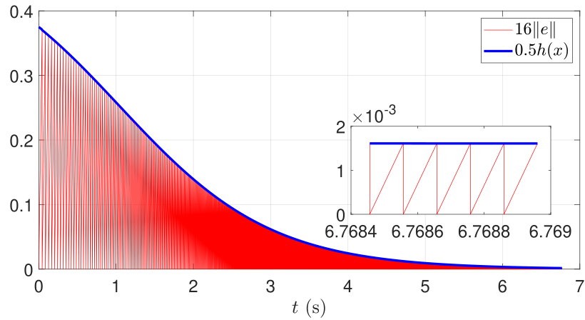
It does not, however, guarantee implementable event spacing. As the barrier approaches zero, the allowable error also vanishes. Motion tangent to the boundary may continue to generate error at a nonvanishing rate, unlike motion approaching an equilibrium. A controller can therefore remain safe while its event intervals shrink toward zero.
Equations 15–18
(15)
(16)
(17)
(18)
IV-A Counterexample
The counterexample is a planar rotating system with an input controlling its radial motion. The safe set is the unit disk, represented by h = 1 − ‖x‖². The stated feedback makes h a valid barrier, and the proposed absolute-value trigger preserves that disk.
The proof assumes a positive MIET and derives a contradiction. Events must continue occurring; the barrier decreases toward zero; yet the rotating state keeps producing sampling error. A Taylor bound then shows that a sufficiently small barrier value forces another event sooner than the assumed minimum interval. The complete derivation and simulation plots are preserved below. This establishes failure of a uniform positive interval, without requiring a claim of finite-time Zeno behavior.
Equations 19–21
(19)
(20)
(21)
Fig. 1: Simulation results for the system (20) using the trigger law (21). Even as the boundary of the safe set is approached , the growth rate of the error does not diminish, leading to arbitrarily small interevent times.
V Event-Triggered Safety
The strong ISSf barrier property adds a fixed positive margin d to the derivative inequality. With zero measurement error, this requires motion strictly into the safe set at its boundary. If the error penalty is Lipschitz with constant L and the relevant dynamics are bounded in norm by F, the proposed trigger guarantees a minimum interval σd/(LF), where 0 < σ ≤ 1. Its tuning function must dominate the barrier comparison function. The theorem also establishes safety and attraction of the certified set under its stated assumptions.
The proof combines two bounds: the trigger maintains the barrier inequality, while bounded dynamics limit how fast sampling error can grow after each reset. Compactness can supply the needed dynamics bound on the relevant state/error region; a stronger domain assumption is needed when claiming attraction from outside. Changing the tuning function can increase actual interevent times without changing the stated uniform lower bound.
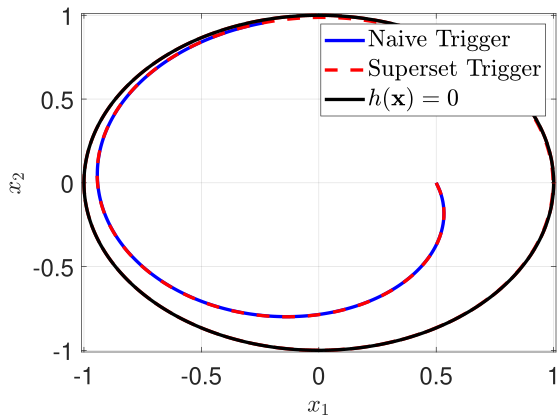
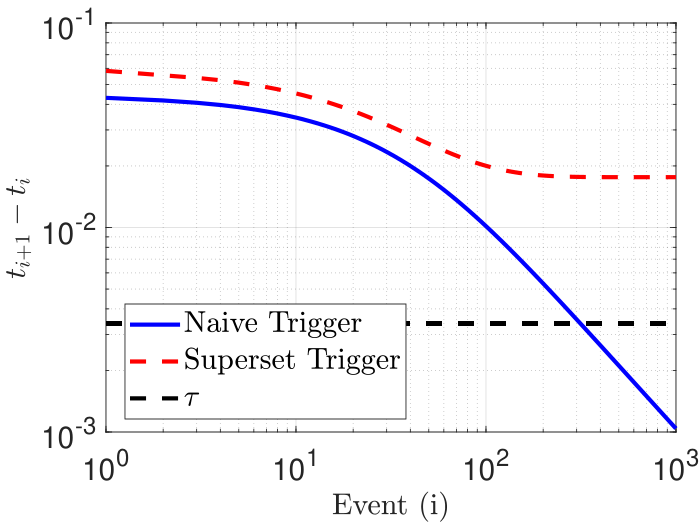
If the original barrier lacks the strong property, replace h by h + b for any positive b. The resulting enlarged set has a positive barrier margin and admits the theorem’s trigger, provided its remaining assumptions hold. Increasing b increases the guaranteed interval but relaxes the original safety boundary. The planar simulations illustrate the contrast: both implementations stay in their certified sets, but only the strengthened construction retains a positive minimum interval.
Equations 22–24
(22)
(23)
(24)
(a)
(b)
(c)
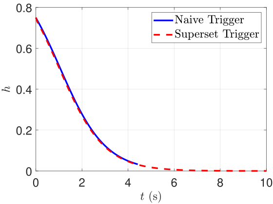
Fig. 2: Simulation results demonstrating safety achieved with an event-triggered controller. (Left) State trajectories for both triggers remain within the safe set for the length of the simulation. (Center) The value of the ISSf-BF remains above zero for the length of the simulation, corresponding to the system remaining safe.
(Right) The interevent times of the two trigger laws. The interevent times of the trigger law (21) approach while the trigger law (V) satisfies the theoretical bound.
Equations 25
(25)
VI Conclusions
The paper separates safe behavior from feasible update timing and links them through a strengthened barrier condition. Its guarantee depends on the stated regularity, boundedness, and barrier assumptions; validation is in simulation. Open directions include choosing the set expansion adaptively, directly constructing strong barriers, and jointly designing triggers for stability and safety.
18 references
[1]
S. Abbott.
Understanding analysis, volume 2.
Springer, 2001.
[2]
A. D. Ames, S. Coogan, M. Egerstedt, G. Notomista, K. Sreenath, and P. Tabuada.
Control barrier functions: Theory and applications.
In European Control Conference (ECC), pages 3420–3431. IEEE,
2019.
[3]
A. D. Ames, X. Xu, J. W. Grizzle, and P. Tabuada.
Control barrier function based quadratic programs for safety critical
systems.
IEEE Transactions on Automatic Control, 62(8):3861–3876, 2017.
[4]
J. Berneburg and C. Nowzari.
Distributed dynamic event-triggered coordination with a designable
minimum inter-event time.
In American Control Conference (ACC), pages 1424–1429.
IEEE, 2019.
[6]
D. P. Borgers and W. P. M. H. Heemels.
Event-separation properties of event-triggered control systems.
IEEE Transactions on Automatic Control, 59(10):2644–2656,
2014.
[7]
W. P. M. H. Heemels, K. H. Johansson, and P. Tabuada.
An introduction to event-triggered and self-triggered control.
In Conference on Decision and Control (CDC), pages 3270–3285.
IEEE, 2012.
[9]
L. Li, X. Wang, and M. D. Lemmon.
Stabilizing bit-rate of disturbed event triggered control systems.
In Conference on Analysis and Design of Hybrid Systems, pages
70–75. IFAC, 2012.
[10]
C. Nowzari, E. Garcia, and J. Cortés.
Event-triggered control and communication of networked systems for
multi-agent consensus.
Automatica, 105:1–27, 2019.
[11]
P. Ong and J. Cortés.
Event-triggered control design with performance barrier.
In Conference on Decision and Control (CDC), Miami Beach, FL,
2018. IEEE.
[12]
R. Postoyan, R.G. Sanfelice, and W. P. M. H. Heemels.
Inter-event times analysis for planar linear event-triggered
controlled systems.
In Conference on Decision and Control (CDC), pages 1662–1667.
IEEE, 2019.
[13]
R. Postoyan, P. Tabuada, D. Nešić, and A. Anta.
A framework for the event-triggered stabilization of nonlinear
systems.
IEEE Transactions on Automatic Control, 60(4):982–996, 2014.
[15]
E. D. Sontag and Y. Wang.
On characterizations of input-to-state stability with respect to
compact sets.
In Nonlinear Control Systems Design, pages 203–208. Elsevier,
1995.
[17]
X. Xu, P. Tabuada, J. W. Grizzle, and A. D. Ames.
Robustness of control barrier functions for safety critical control.
IFAC-PapersOnLine, 48(27):54–61, 2015.
[18]
G. Yang, C. Belta, and R. Tron.
Self-triggered control for safety critical systems using control
barrier functions.
In American Control Conference (ACC), pages 4454–4459.
IEEE, 2019.