At a glance
Intuition. Think of WeightWatcher as a checkpoint inspection dashboard. It summarizes weight matrices to flag unusual layers or compare trends among models, much as component measurements can flag hardware for further testing. Those measurements do not replace testing the complete system.
Reading the math. For the unnormalized matrix X=WᵀW, each eigenvalue λ is a squared stretching strength. Their sum gives ‖W‖²_F, the total squared weight size; λ_max gives the strongest direction. The fitted exponent α describes how quickly the spectral tail thins out. Multiplying W by two multiplies every λ by four, illustrating why scale and normalization matter. Computing these statistics needs only weights; judging their usefulness requires performance evidence.
WeightWatcher evaluates pretrained models through their weight spectra without needing the original training or test examples at inspection time. The paper compares average log norms with fitted power-law metrics across computer-vision and language-model series. Norms often track reported accuracy within familiar model families; fitted exponents and scale-weighted exponents sometimes discriminate trends better and expose unusual layers. The evidence is an observational meta-analysis using externally reported performance, not a data-free guarantee of correctness, robustness, or generalization. Several source-table and notation inconsistencies are retained and qualified below.
1 Introduction
A model user may have weights but little knowledge of the data or training recipe. The proposed diagnostic extracts information from those weights rather than retraining or rerunning a benchmark. It aims to predict relative trends across pretrained models and identify suspicious layer behavior, rather than derive a generalization bound or introduce a new regularizer. The analysis combines familiar matrix norms with heavy-tailed self-regularization metrics [Martin and Mahoney, 2018; Martin and Mahoney, 2019]. The authors’ term “quality” mainly refers to agreement with reported accuracy trends and their spectral interpretation; the study does not directly measure fairness, safety, or robustness.
2 Results
The results progress from the metric definitions to detailed vision and language examples, then to a broader collection of architecture–dataset regressions. Within-family comparisons and cross-architecture diagnoses have different limitations and should not be treated as interchangeable.
2.1 Overall approach
The network’s weights and biases determine a prediction function, so its parameter structure can be inspected without examples. WeightWatcher version 0.2.7 computes the reported diagnostics from public checkpoints. The researchers do not train the models or independently reproduce their reported test accuracies; those external numbers supply the comparison target. Consequently, “without data” describes computing the proposed metric, not validating its relationship with performance without any performance information.
Equations 1–2
| (1) |
| (2) |
Metrics for DNN Weight Matrices.
Each analyzed two-dimensional matrix contributes Gram eigenvalues λᵢ, the squares of its singular values. The metrics are squared Frobenius size, largest eigenvalue, a fitted exponent multiplied by log λ_max, and a power sum of eigenvalues related to a Schatten norm. The source’s Equation 3 has a notation error: for X=WᵀW, ∑λᵢ=tr(X)=‖W‖²_F, whereas ‖X‖_F=√∑λᵢ² in general. Its displayed equality is preserved. Equation 4 uses the symbol ∞ for the spectral/operator norm, not the usual maximum-row-sum induced infinity norm. These conventions matter when reproducing the metrics.
Equations 3–6
| Frobenius Norm: | (3) | ||
| Spectral Norm: | (4) | ||
| Weighted Alpha: | (5) | ||
| -Norm (or -Shatten Norm): . | (6) |
Overview of Heavy-Tailed Self-Regularization.
Heavy-tailed self-regularization interprets broad weight spectra as signatures of learned correlations. A bounded-range power-law fit ρ(λ)∝λ⁻α summarizes the empirical spectrum. Smaller fitted α is hypothesized to indicate stronger multiscale structure in the relevant regime. This interpretation does not establish a unique learning mechanism, actual mutual information, or a universal “smaller is better” theorem. The paper discusses self-organized criticality and multiplicative optimization noise as possible explanations without selecting one. It introduces a normalized Gram matrix for the theoretical discussion; the empirical normalization rules later explain why practical weights are mostly used as stored.
Equations 7
| (7) |
DNN Empirical Quality Metrics.
Model-level metrics average layer log norms or α·log λ_max. The unweighted average α is proposed for identifying unusual models when scale-dependent quantities behave misleadingly. Power-law fitting selects a lower cutoff by minimizing Kolmogorov–Smirnov distance, following the cited maximum-likelihood methodology [Clauset et al., 2009; Alstott et al., 2014]. Large fitted exponents and weak fits require caution. Uniform rescaling changes norms and weighted α but ideally leaves the exponent unchanged.
The product-norm analogy motivates these aggregates; averaging over layers of different depths is an empirical convention, not itself a generalization bound. The weighted exponent approximates the log power sum only when the non-leading eigenvalues contribute little enough: for positive α, their difference lies between zero and log M for M eigenvalues. Equation 13 prints λᵅ, while Equation 7 and the surrounding description use the decaying law λ⁻α. Both original displays are retained; this is a source sign inconsistency, not evidence about the software implementation.
Equations 8–13
| (8) |
| (9) |
| (10) |
| (11) |
| (12) |
| (13) |
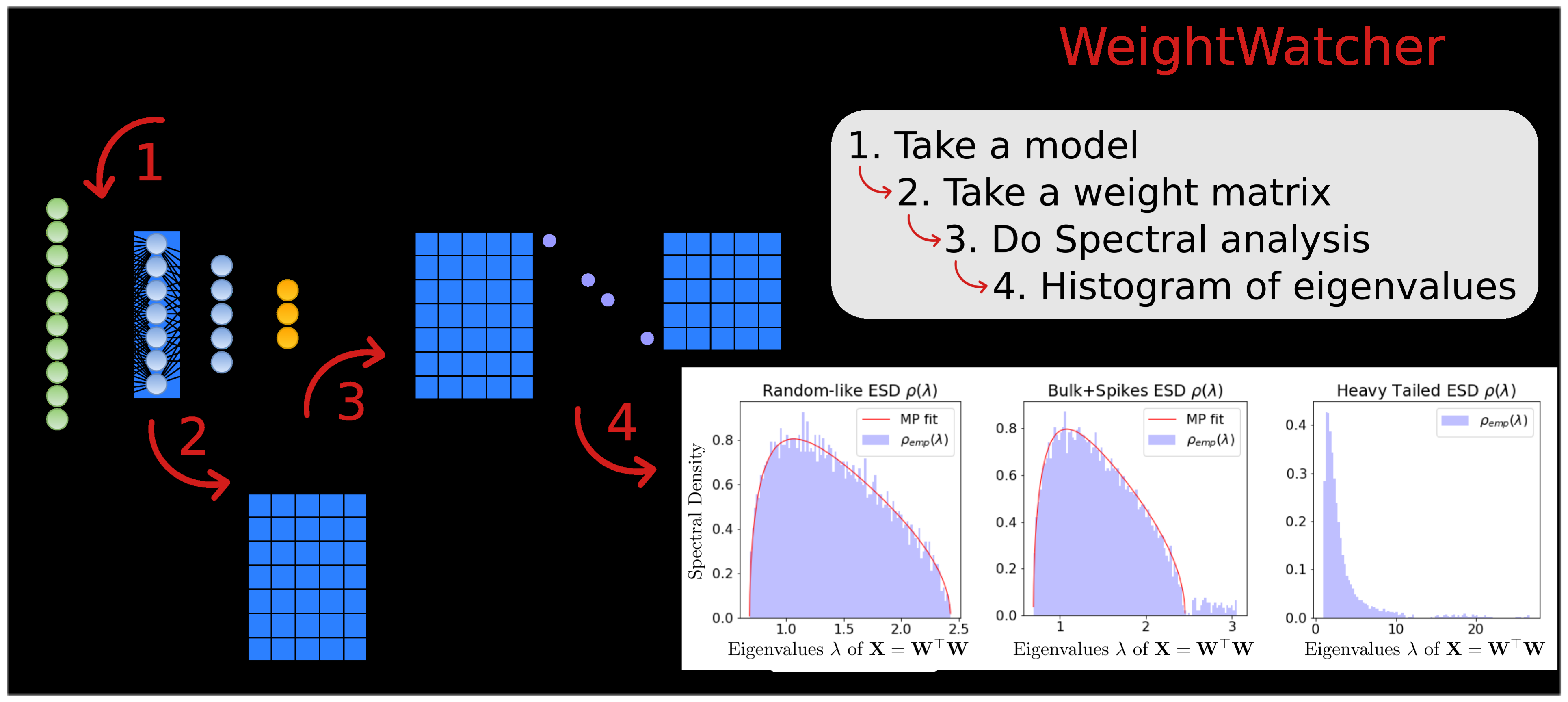
2.2 Comparison of CV models
The detailed vision comparisons use public VGG, ResNet, DenseNet, and a separate OSMR ResNet checkpoint series labeled “ResNet-1K.” They compare model-level accuracy trends and layer-level spectral behavior. Repository, architecture, training recipe, and checkpoint differences remain potential confounders.
Average Quality Metrics versus Reported Test Accuracies.
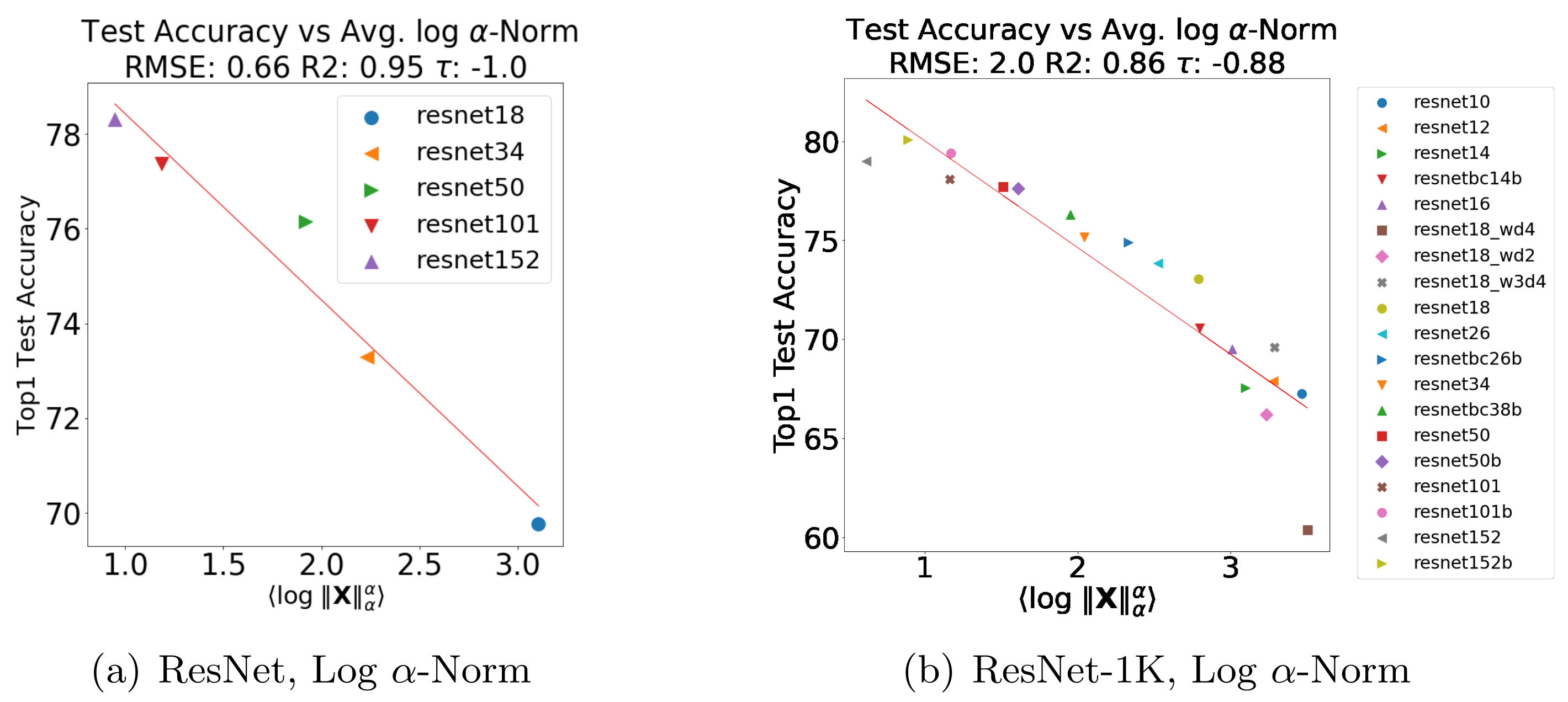
All four metrics correlate with reported performance in the small familiar model series. The spectral norm has the best reported VGG fit, with RMSE 0.23 and R² 0.98. Weighted α performs best among the listed ResNet metrics, with RMSE 0.61 and R² 0.96; for the separate ResNet-1K series its RMSE is 1.8 and R² 0.89. Thus the evidence favors different metrics in different families, not a uniform victory for power-law metrics. Table 1 and all regression plots retain their exact numbers.
The source interprets the ResNet/ResNet-1K contrast as a training-set-size comparison. The checkpoint comparison by itself does not establish that causal explanation, and ordinary ImageNet classification checkpoints also commonly use the 1,000-class benchmark. These series should therefore be read as distinct checkpoint collections unless their actual training-data differences are independently established. Reported accuracies are taken as given, and the fitted regressions are not a held-out prediction experiment.
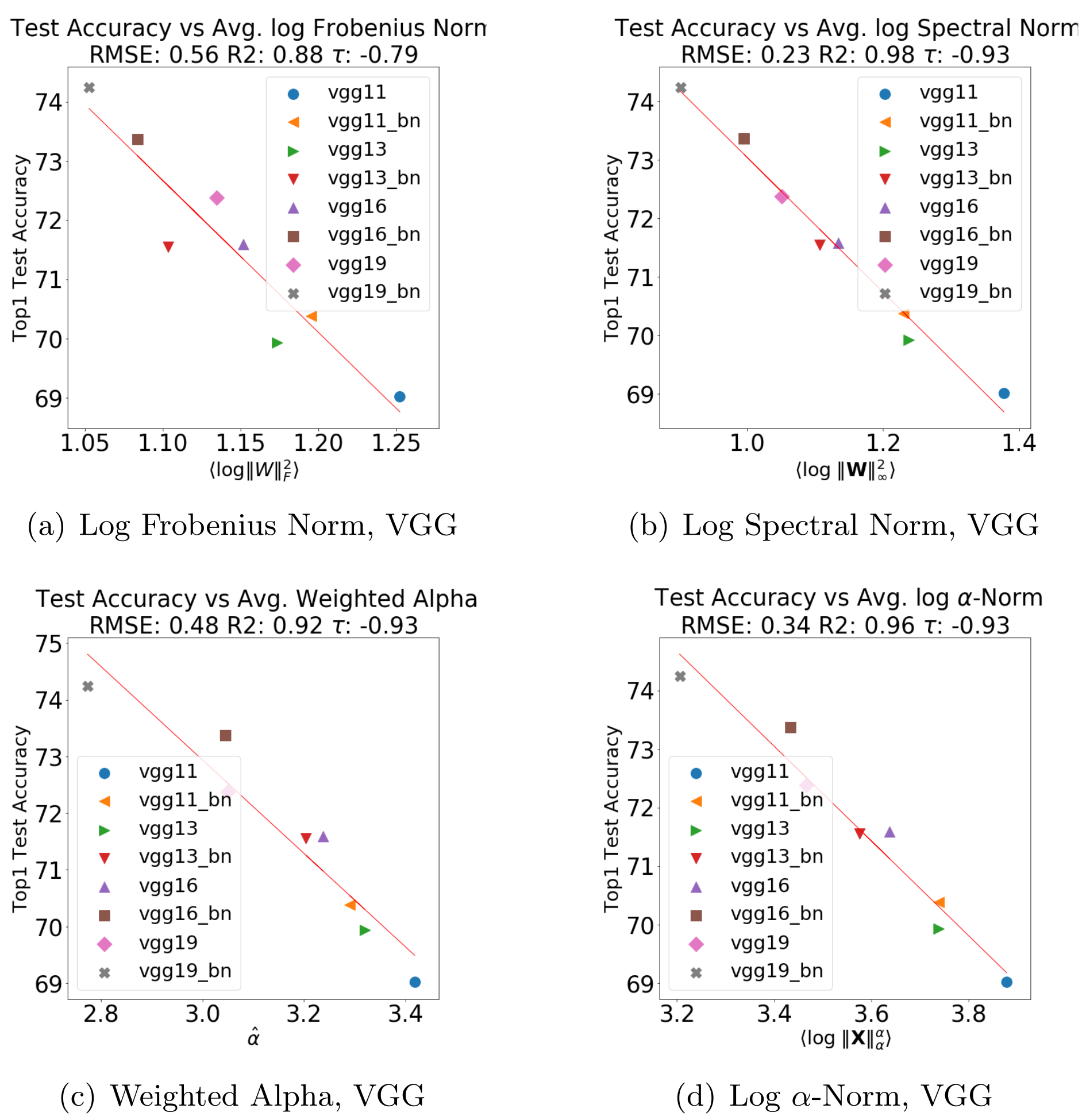
| Series | # | Metric | ||||
| VGG | 6 | RMSE | 0.56 | 0.23 | 0.48 | 0.34 |
| 0.88 | 0.98 | 0.92 | 0.96 | |||
| Kendall- | -0.79 | -0.93 | -0.93 | -0.93 | ||
| ResNet | 5 | RMSE | 0.9 | 0.97 | 0.61 | 0.66 |
| 0.92 | 0.9 | 0.96 | 0.9 | |||
| Kendall- | -1.0 | -1.0 | -1.0 | -1.0 | ||
| ResNet-1K | 19 | RMSE | 2.4 | 2.8 | 1.8 | 1.9 |
| 0.81 | 0.74 | 0.89 | 0.88 | |||
| Kendall- | -0.79 | -0.79 | -0.89 | -0.88 | ||
| DenseNet | 4 | RMSE | 0.3 | 0.11 | 0.16 | 0.21 |
| 0.93 | 0.99 | 0.98 | 0.97 | |||
| Kendall- | -1.0 | -1.0 | -1.0 | -1.0 |
Layer Analysis: Metrics as a Function of Depth.
Layerwise α differs substantially by architecture. In VGG, exponents generally rise through convolutional layers and fall in the final fully connected layers. The deeper examined ResNet has a long region of relatively stable exponents near two; DenseNet shows more variable and sometimes much larger values. Figure 4 retains the distinct vertical-axis ranges and overlaid-layer comparison. These patterns motivate architecture-specific diagnostics and the authors’ explicit warning against treating cross-architecture metric values as directly comparable.
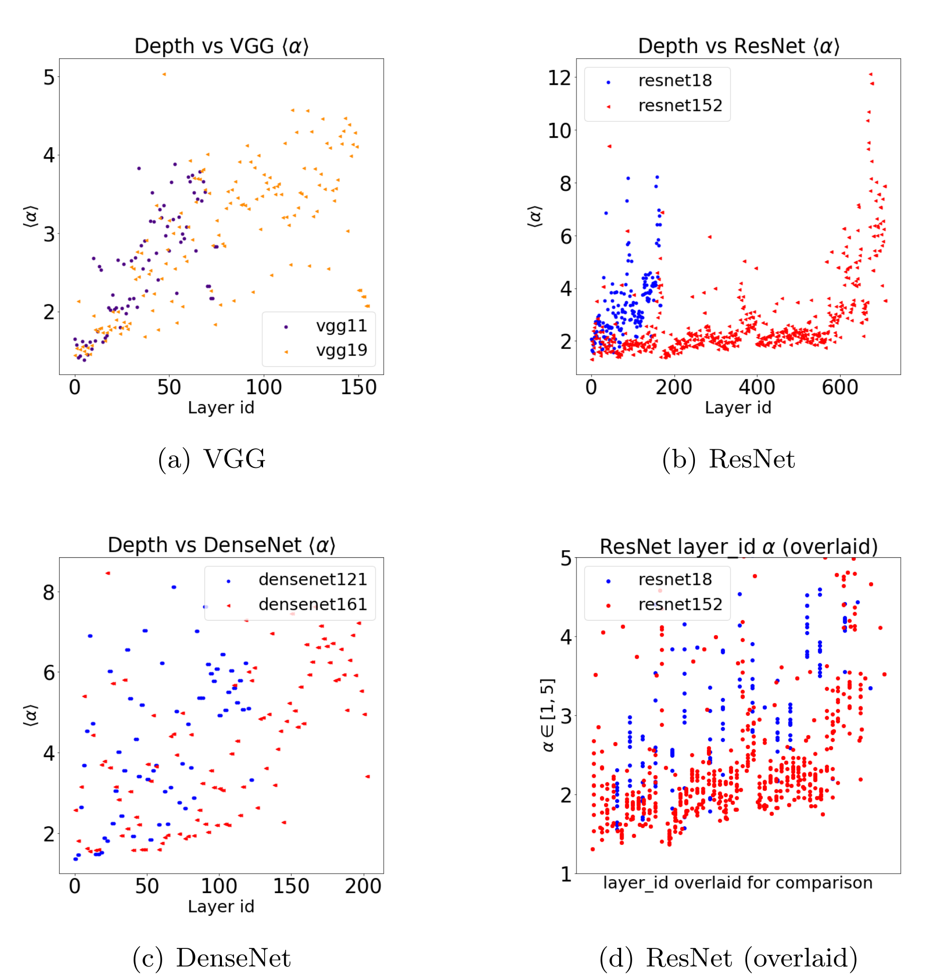
Correlation Flow; or How α Varies Across Layers.
“Correlation flow” names the hypothesis that small, relatively stable exponents across successive layers reflect useful propagation of learned structure. It is inferred from weight spectra, not measured by passing data through the network or estimating information transfer. Large α may instead indicate a poor power-law model. The analogy to information-bottleneck work is conceptual; these diagnostics do not calculate the same mutual-information quantities.
Scale Collapse; or How Distillation May Break Models.
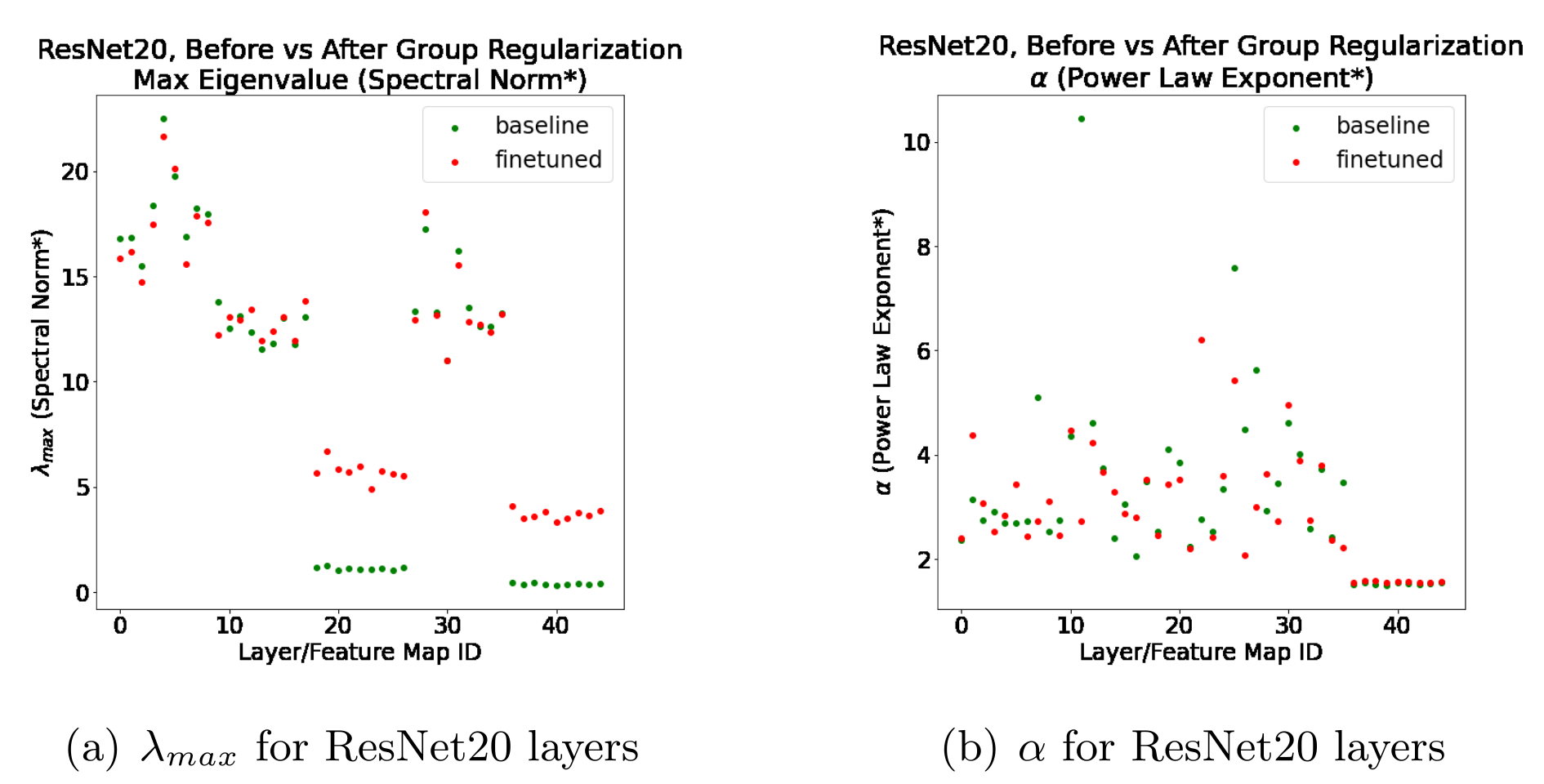
For a group-regularized ResNet20 checkpoint, reported Top1 accuracy falls from 91.45 to 91.02 and Top5 from 99.75 to 99.67 after compression/fine-tuning. Norms do not follow the simple expected accuracy ordering. The authors call strongly uneven changes in layer scale “scale collapse” and inspect α separately; some very large baseline exponents disappear after compression, while other aggregate indicators worsen. This is a useful counterexample to reading smaller norms as automatically better. The claim that distillation has “damaged” internal information is an interpretation of these diagnostics and a small reported accuracy change, not an independently measured failure mechanism. The subsection also describes the scale anomaly in both increasing- and decreasing-norm terms; Figure 5 preserves the actual layerwise comparison.
2.3 Comparison of NLP Models
Transformer checkpoints contain larger and differently structured matrices than the vision examples. The paper interprets unusually large fitted α as possible undertraining relative to model size, while acknowledging that the power-law fit is less reliable in this regime. Such values can flag a spectrum for inspection, but do not uniquely distinguish insufficient data, optimization, architecture, or an unsuitable distributional fit. Embedding layers need separate treatment because their normalization differs.
OpenAI GPT Models.
The language examples compare GPT with GPT2-small and then GPT-2 models of increasing size. These are historical checkpoints obtained through the cited Hugging Face tooling [Wolf et al., 2019]. Table 2 retains the analyzed matrix counts and model-level metrics; embeddings are omitted from those averages. GPT and GPT-2 differ in embeddings, context sizes, data, and training details, so the comparison is not a controlled change in data quality alone. The source’s account of release motives and its labels “deficient” and “well-trained” should not be taken as facts established by the weight-spectrum analysis.
| Series | # | ||||
| GPT | 49 | 1.64 | 1.72 | 7.01 | 7.28 |
| GPT2-small | 49 | 2.04 | 2.54 | 9.62 | 9.87 |
| GPT2-medium | 98 | 2.08 | 2.58 | 9.74 | 10.01 |
| GPT2-large | 146 | 1.85 | 1.99 | 7.67 | 7.94 |
| GPT2-xl | 194 | 1.86 | 1.92 | 7.17 | 7.51 |
Average Quality Metrics for GPT and GPT2.
From GPT2-medium to large to xl, most reported scale-dependent metrics decrease, broadly matching the expected model-quality ordering. GPT2-small does not follow that ordering exactly. All four aggregate metrics increase from GPT to GPT2-small, opposite the proposed simple smaller-is-better rule. This motivates decomposing weighted α into scale and exponent instead of trusting one model score. The analysis does not provide a universal calibration from metric value to downstream accuracy.
Layer Analysis: Scale Collapse in GPT and GPT2.
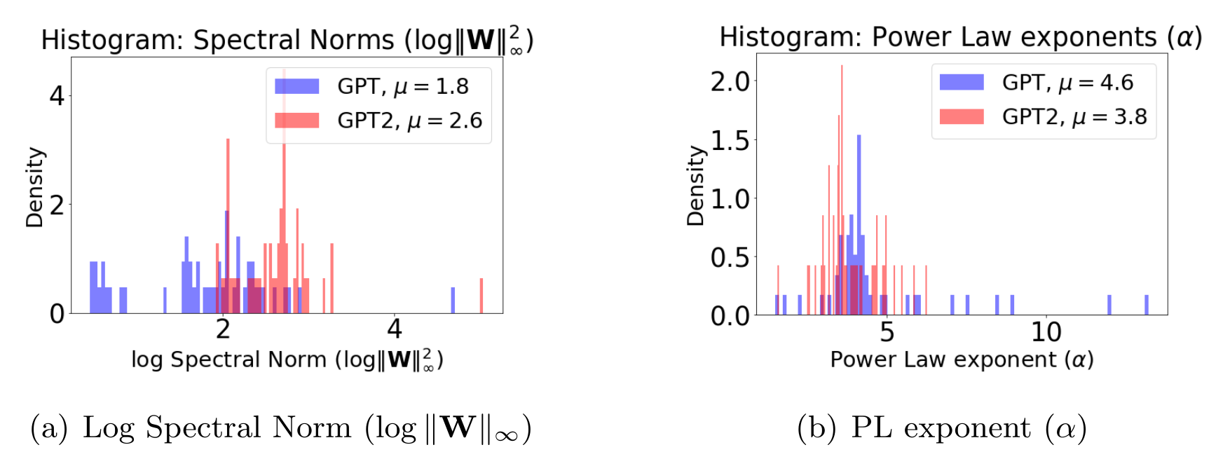
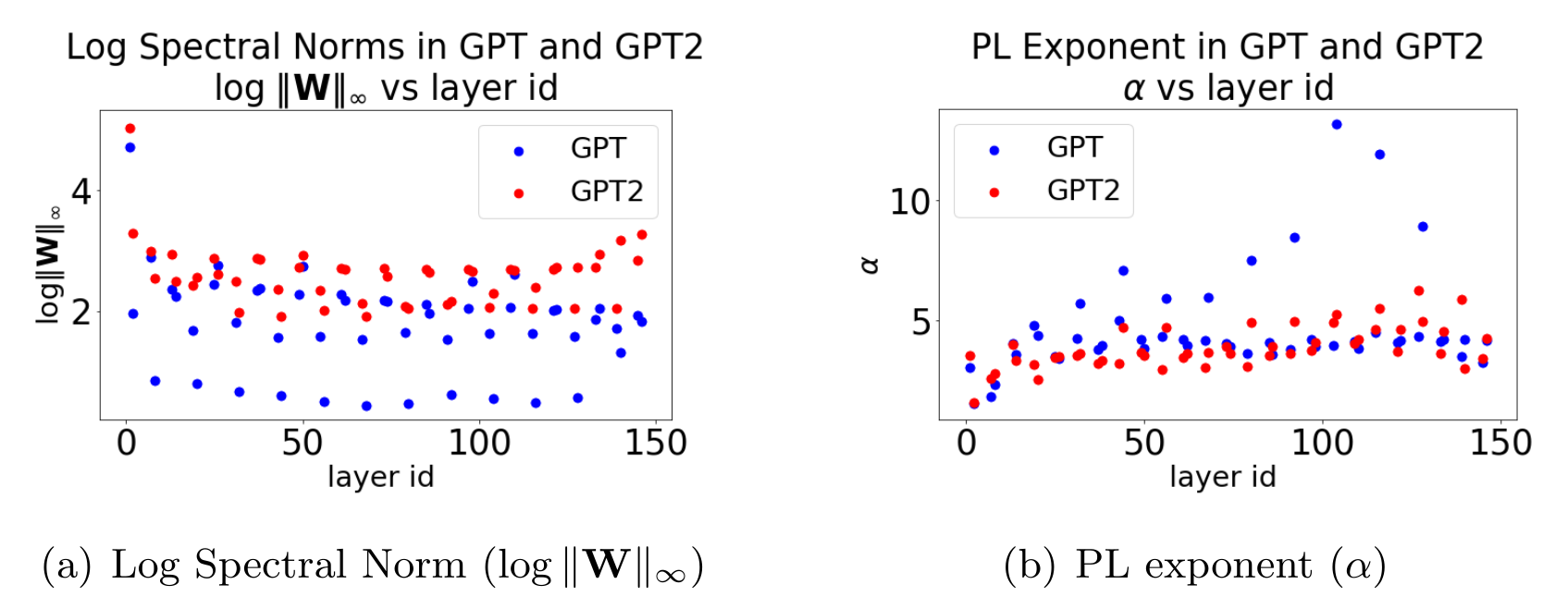
GPT has more very small layer spectral norms than GPT2-small, while embeddings produce exceptionally large values due to their different scale. Figure 7 shows alternating layer types rather than one homogeneous sequence. The authors interpret the older model’s low norms as scale collapse, illustrating why a norm can be smaller for a less capable checkpoint. Embeddings are retained in diagnostic plots but excluded from the stated aggregate comparison.
Layer Analysis: Correlation Flow in GPT and GPT2.
GPT2-small has fewer unusually large fitted exponents than GPT and more stable layerwise patterns. The unweighted exponent average therefore follows the authors’ expected ordering where weighted metrics do not. This is evidence that separating scale from spectral shape can be useful. Calling the pattern better “correlation flow” remains a hypothesis about learned structure, rather than a direct measurement of information retained or a proof of causal improvement.
GPT2: medium, large, xl.
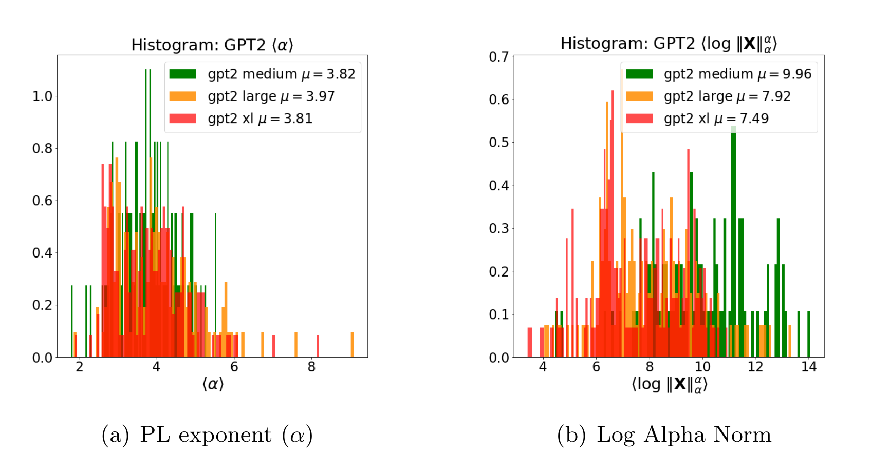
The larger GPT-2 comparisons show lower scale-dependent metrics overall, while the exponent distributions have mixed changes. The text reports mean α values 3.82, 3.97, and 3.81 for medium, large, and xl: these are not monotonically decreasing despite the accompanying monotonic description. Some large-exponent tails grow in larger models. The suggestion that those models could benefit from more data or optimization is plausible as a hypothesis, but the spectrum alone does not establish a compute-optimal data requirement or identify which intervention will help.
2.4 Comparing Hundreds of Models
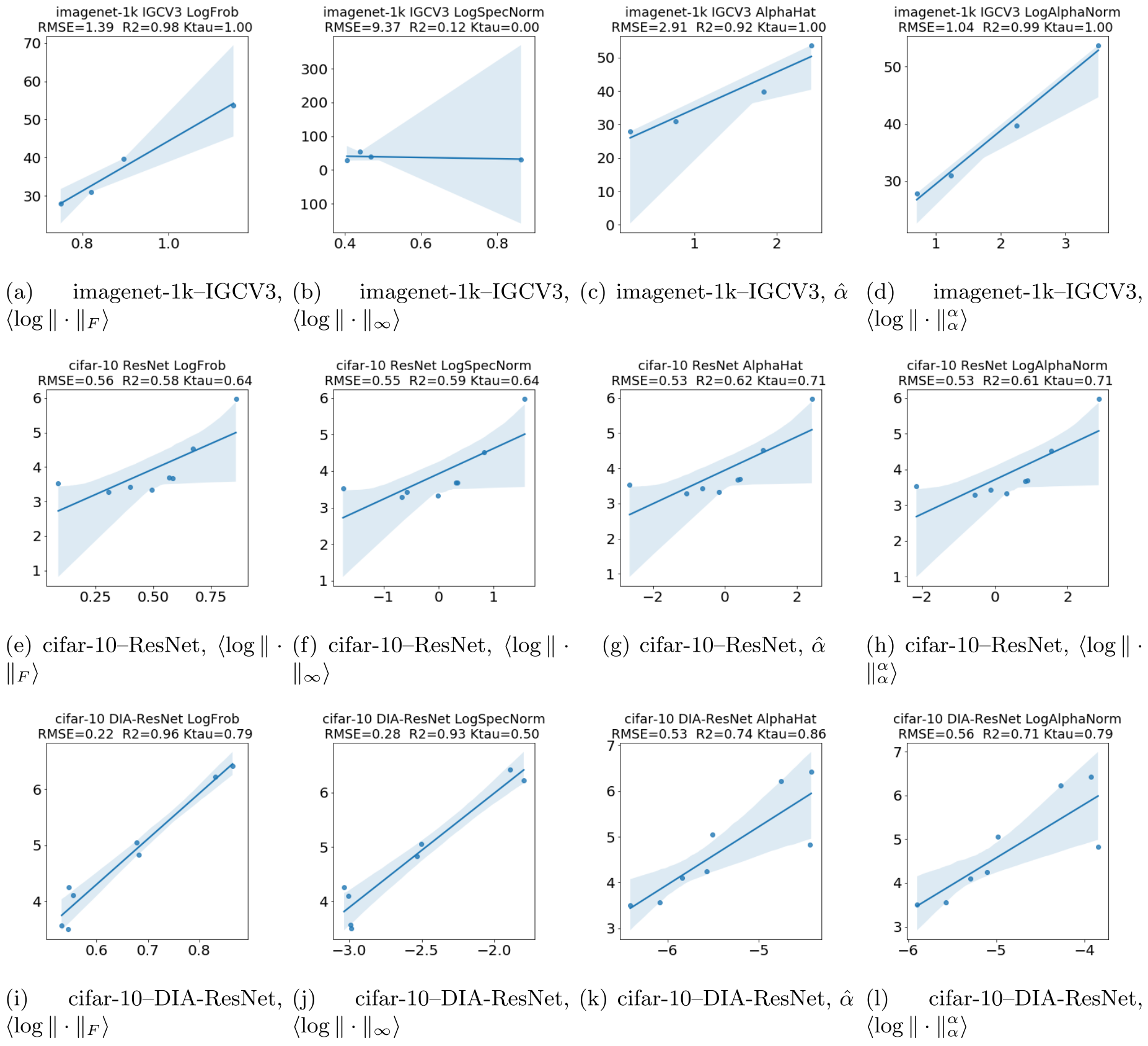
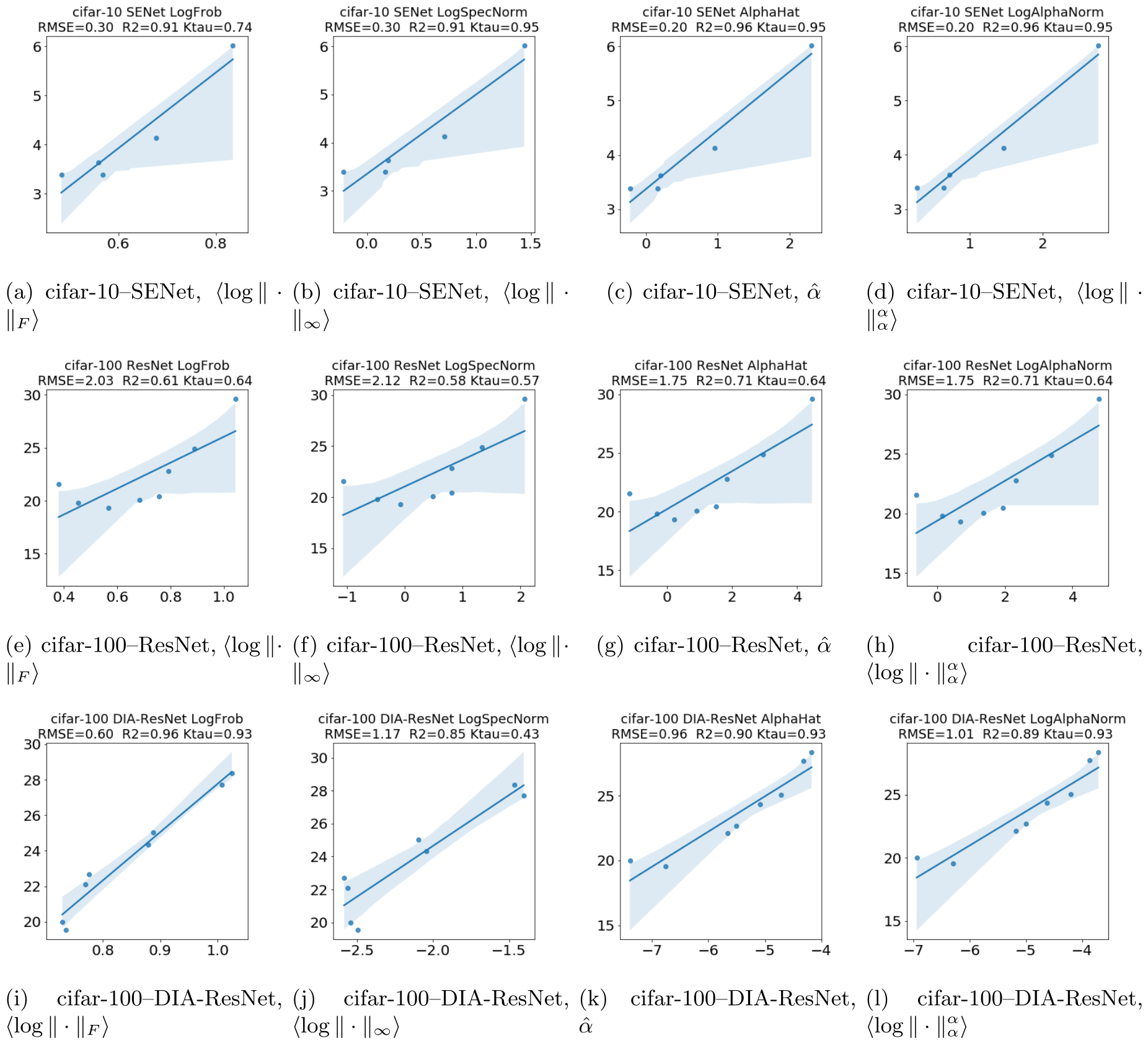
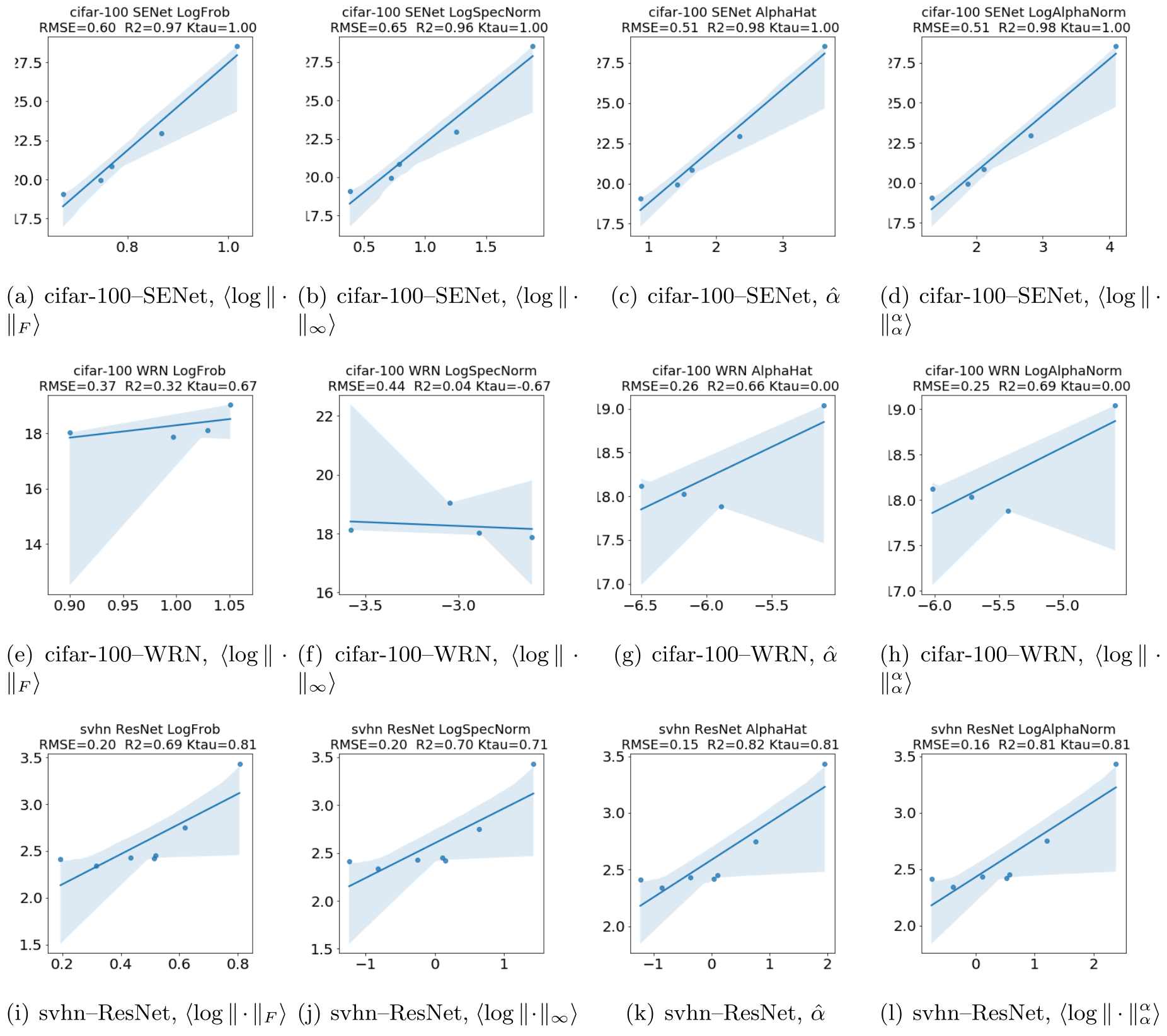
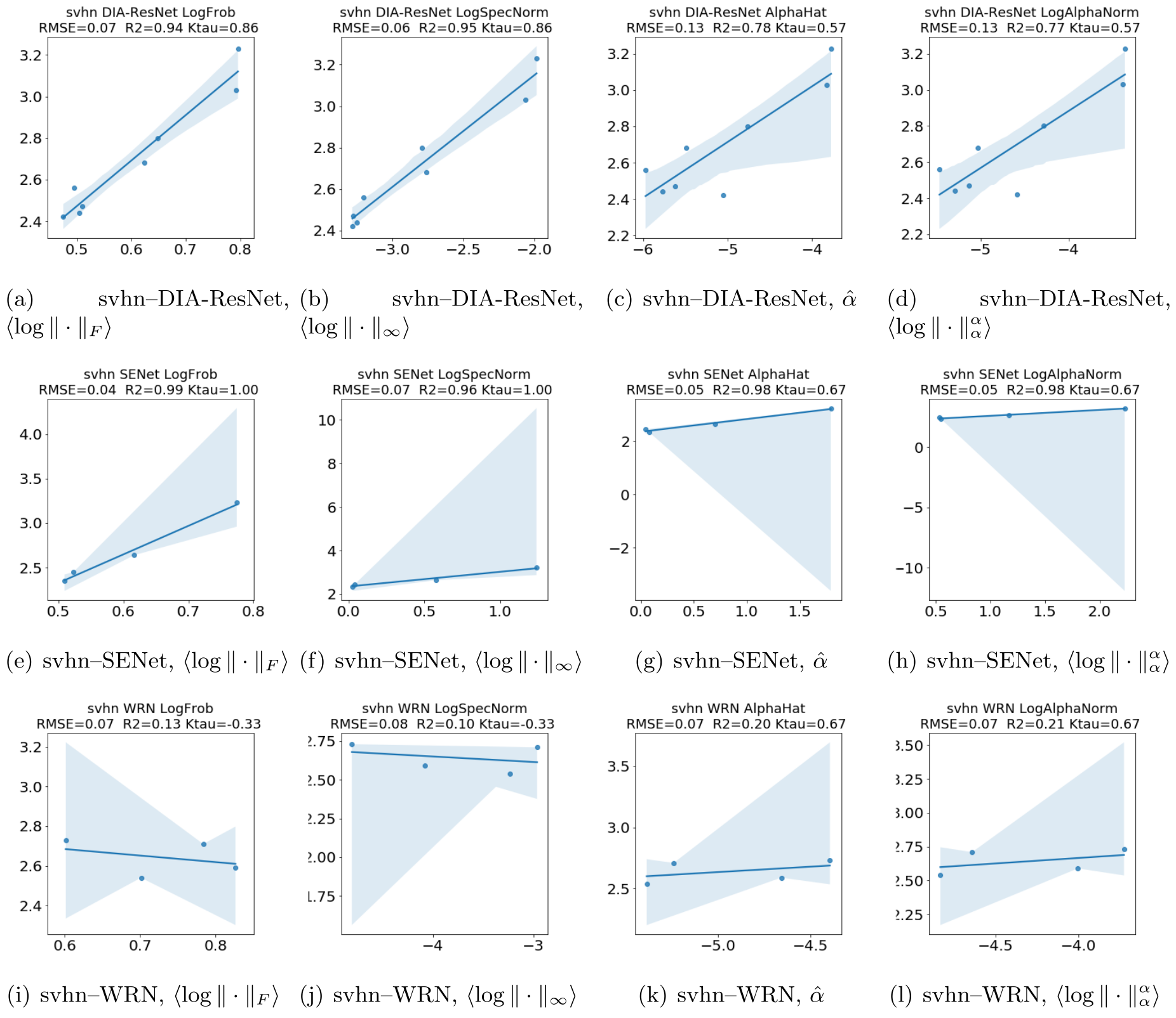
The broad analysis fits separate regressions between weight metrics and reported performance for architecture–dataset groups. Tables 6–8 and Figures 9–17 provide the detailed evidence, including weak or reversed relationships. Selection rules retain particular series and omit several datasets/outliers, so this is not an unbiased census of all possible checkpoints.
Table 3 contains an unresolved numerical inconsistency in the exact v2 PDF: mean R² values are about 3.9 and mean Kendall τ values about 3.8, outside the stated metrics’ permissible upper bounds. Its standard deviations near 9 are also inconsistent with ordinary bounded correlation summaries. The table is preserved exactly, but its aggregate numbers cannot substantiate the claimed overall ranking without correction. The caption describes 108 models, whereas the appendix calls these 108 regressions and Table 5 lists 211 models; those quantities should not be conflated.
| RMSE (mean) | 4.84 | 5.57 | 4.58 | 4.55 |
| RMSE (std) | 9.14 | 9.16 | 9.16 | 9.17 |
| R2 (mean) | 3.9 | 3.85 | 3.89 | 3.89 |
| R2 (std) | 9.34 | 9.36 | 9.34 | 9.34 |
| Kendal-tau (mean) | 3.84 | 3.77 | 3.86 | 3.85 |
| Kendal-tau (std) | 9.37 | 9.4 | 9.36 | 9.36 |
3 Discussion
Comparison of VGG, ResNet, and DenseNet Architectures.
The authors connect stable ResNet exponents with residual connections and interpret erratic DenseNet exponents as excessive connectivity or weaker optimization. These are architecture-design hypotheses derived from selected spectra. The study does not ablate connections while holding training and other architecture choices fixed, so it does not establish that DenseNet’s connectivity itself is harmful.
Related work.
The approach draws on statistical mechanics, random-matrix models, and norm-based complexity measures. Its empirical purpose differs from proving a capacity bound or designing a regularizer. It also differs from information-bottleneck analysis because it inspects stored weights without data-dependent information estimates. The paper relates its results to contemporary weight-only model-quality studies, while arguing that breadth of architectures and model scale matter for extrapolating their conclusions.
Conclusions.
The practical contribution is a reproducible framework for inspecting pretrained weight spectra and comparing several candidate diagnostics. Selected within-family trends support using these metrics as screening signals, with spectral shape sometimes adding information beyond norm scale. They do not replace evaluation on the intended task, resolve the source’s aggregate-table anomaly, or certify that a flagged layer needs a particular repair.
Looking forward.
The authors advocate a semi-empirical theory that combines asymptotic ideas with fitted finite-model parameters. Such an approach can organize observations and generate testable predictions. Its usefulness still depends on fit quality, normalization conventions, selection effects, and validation on models outside the fitted series; a theoretical analogy alone does not establish those predictive properties.
4 Methods
The study uses public pretrained checkpoints and WeightWatcher version 0.2.7. Its accompanying notebooks specify model extraction, spectral fitting, and regression analysis. Reproduction requires matching those historical checkpoint and software conventions, rather than assuming current releases are identical.
Additional Details on Layer Weight Matrices
Linear layers contribute one two-dimensional weight matrix. A convolutional kernel contributes one channel matrix for each spatial kernel location. Biases and much of the surrounding computation—normalization, nonlinearities, residual routing, and other architectural structure—are omitted from this analysis. The resulting collection is therefore a parameter diagnostic, not a full description of the network’s function.
SVD of Convolutional 2D Layers.
The methods distinguish separate SVDs of spatial kernel slices, an SVD of a stacked kernel, and Fourier-domain convolution analysis. The paper chooses separate slice SVDs for speed and reproducibility across thousands of matrices. These spectra are not generally the singular spectrum of the complete convolution operator. Results depend on this extraction convention.
Normalization of Empirical Matrices.
Empirical weights are largely used at their stored scale, relying on initialization conventions rather than explicitly dividing every Gram matrix by N. Convolutional slices are rescaled by k/√2 to align the chosen convention with fully connected layers. Exponents are intended to be invariant under uniform scale changes, while norms and weighted exponents are not. The source’s discussion uses σ² alongside square-root initialization scalings, mixing variance and standard-deviation notation; exact normalization should be checked in the stated software rather than inferred from that prose alone.
Special consideration for NLP models.
Token and position embeddings can have much larger Gram eigenvalues than other transformer matrices because their normalization differs. The authors inspect them as stored, while excluding the first embedding matrices from the headline language-model averages. This distinction must be maintained when reproducing tables or comparing model scores.
Acknowledgements.
The acknowledgements list research support and discussions concerning group regularization. The authors state that the conclusions do not imply sponsor endorsement.
Data availability.
The analyzed models are public, and the generated datasets are provided with the analysis repository. Availability supports inspection of the reported fits; it does not mean their benchmark accuracies were independently remeasured here.
Code availability.
The accompanying ww-trends-2020 repository contains code and notebooks for the reported analysis.
Appendix A Supplementary Information
A.1 Supplementary Details
Reproducing Sections 2.2 and 2.3 .
Table 4 maps the detailed vision and language comparisons to their notebooks, including separate VGG, ResNet, DenseNet, GPT, GPT-2, and broad OSMR analyses. The provided model distributions and versioned tooling define the intended reproduction target.
| Table | Figure | Jupyter Notebook |
| 1 | 2 | WeightWatcher-VGG.ipynb |
| 1 | 3(a) | WeightWatcher-ResNet.ipynb |
| 1 | 3(b) | WeightWatcher-ResNet-1K.ipynb |
| 1 | 4(a) | WeightWatcher-VGG.ipynb |
| 1 | 4(b) | WeightWatcher-ResNet.ipynb |
| 1 | 4(c) | WeightWatcher-DenseNet.ipynb |
| 5 | WeightWatcher-Intel-Distiller-ResNet20.ipynb | |
| 2 | 6 | WeightWatcher-OpenAI-GPT.ipynb |
| 2 | 7, 8 | WeightWatcher-OpenAI-GPT2.ipynb |
| 3,7,8,9 | Appendix | OSMR-Analysis.ipynb |
Reproducing Figure 5 , for the Distiller Model.
The distiller folder supplies the original group-regularization notebooks for Figure 5 and additional compressed-model examples. The baseline and modified checkpoint identities matter because the comparison concerns their actual stored parameters.
Reproducing Table 3 in Section 2.4 .
The broad corpus was collected in January 2020 using WeightWatcher 0.2.7. Later software can use the stated compatibility option, but public checkpoints may change. The appendix describes excluding datasets with few models, regressions with fewer than five points, two visually identified EfficientNet outliers, and the CIFAR-100 ResNeXt series that lacked the desired norm trend. These exclusions affect the interpretation of a global performance claim.
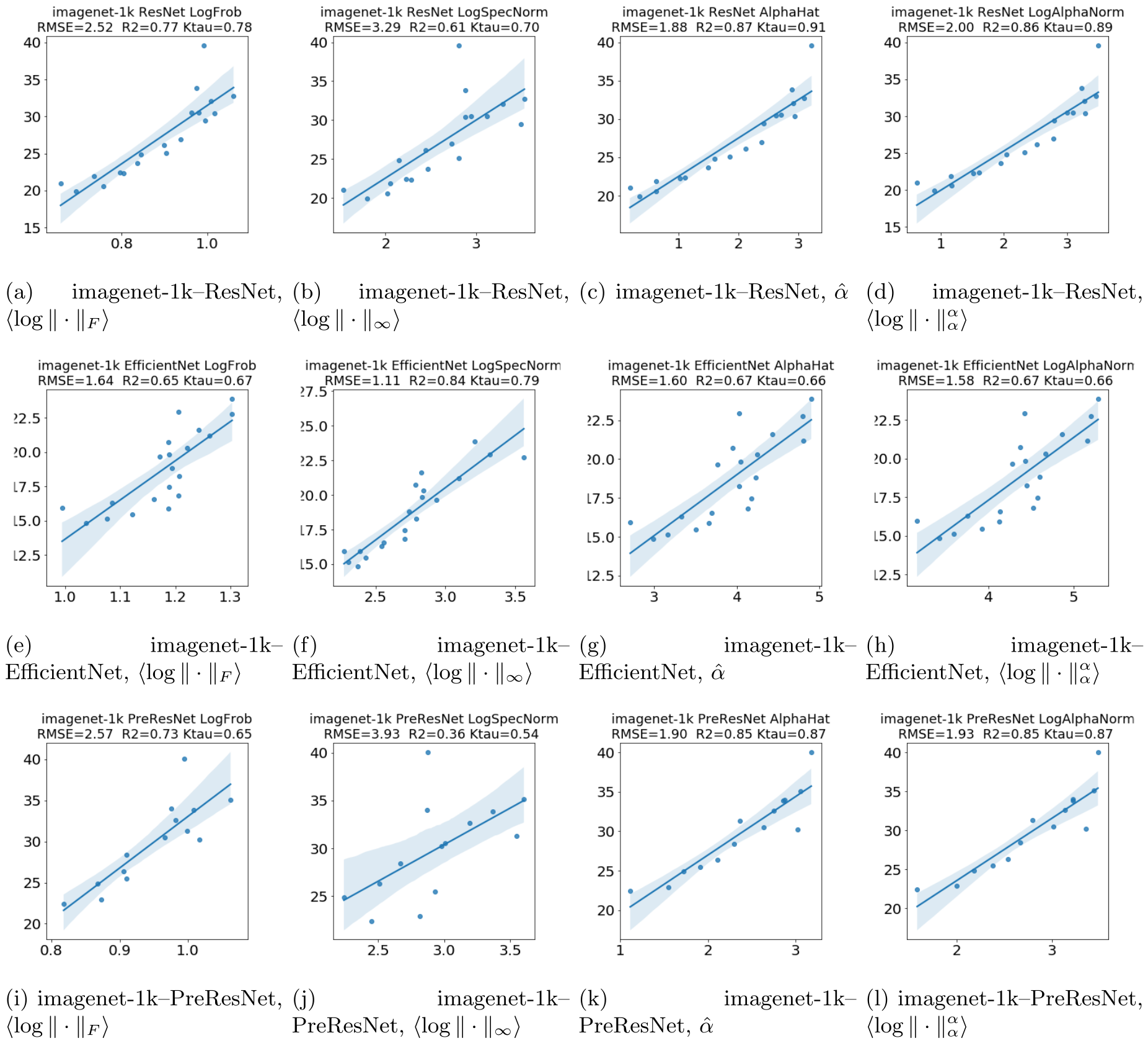
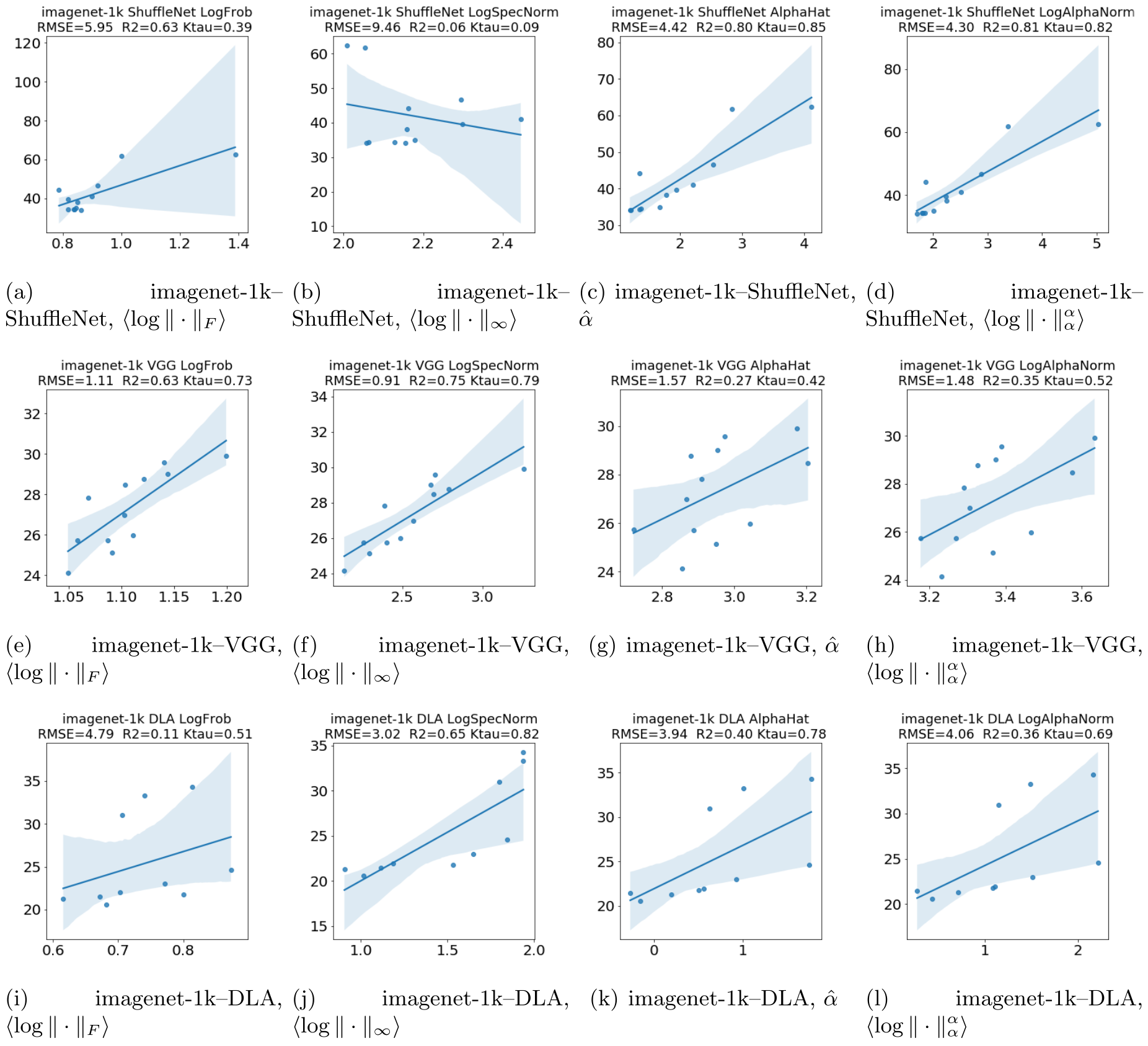
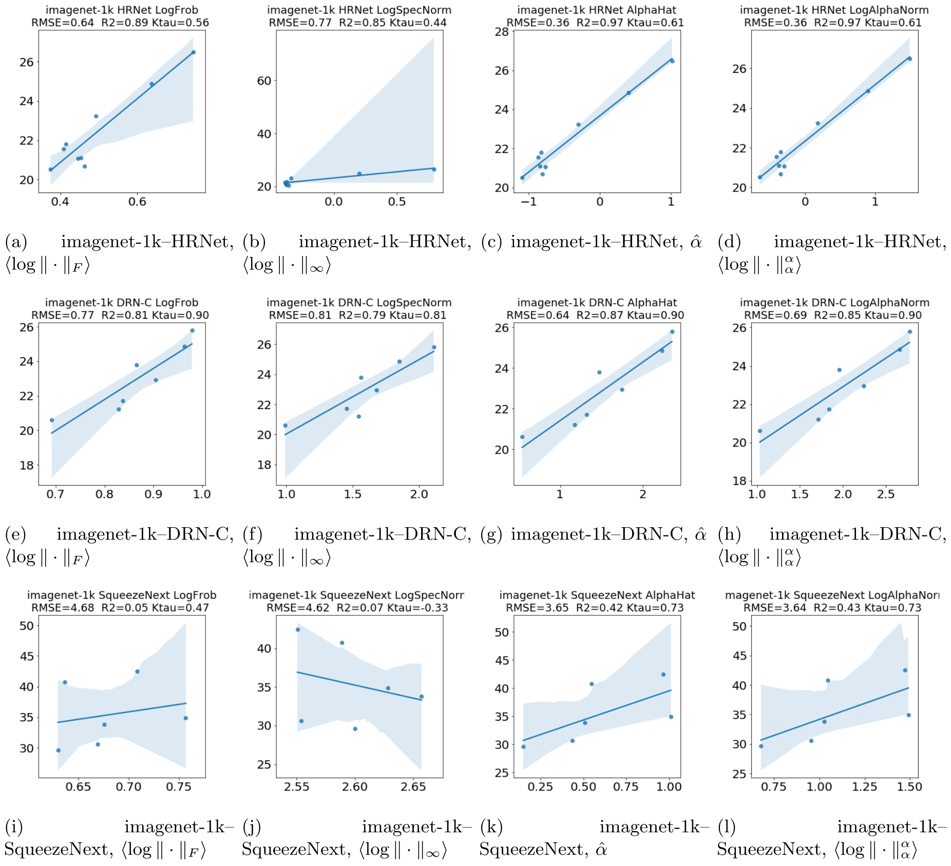
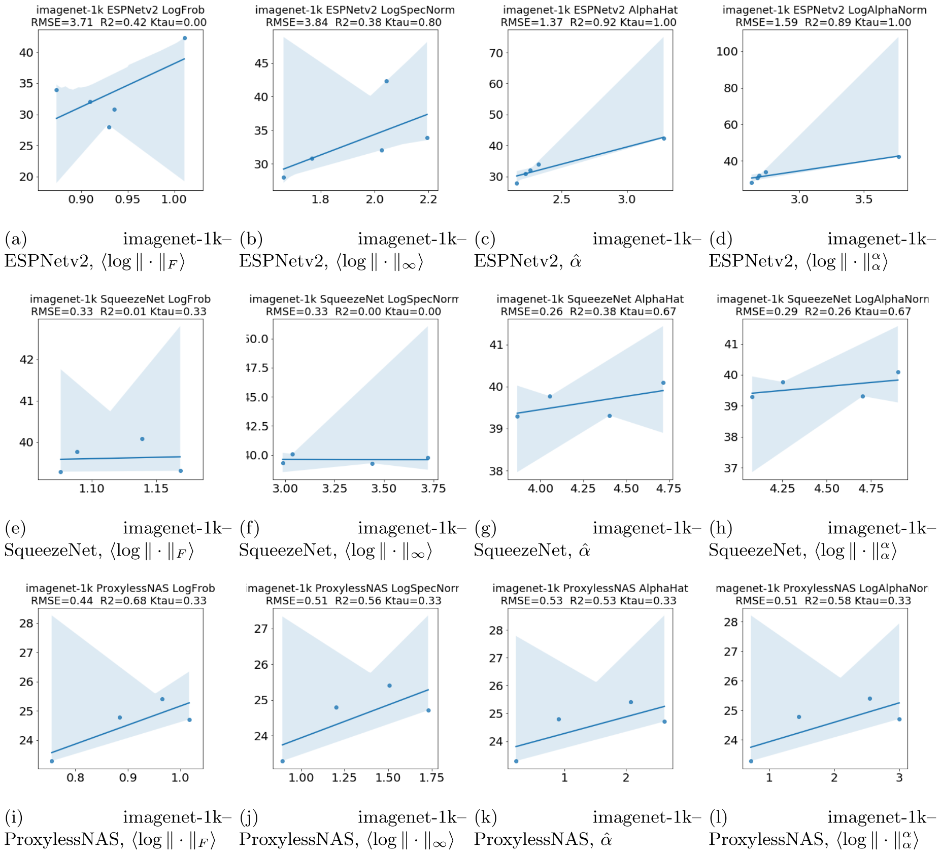
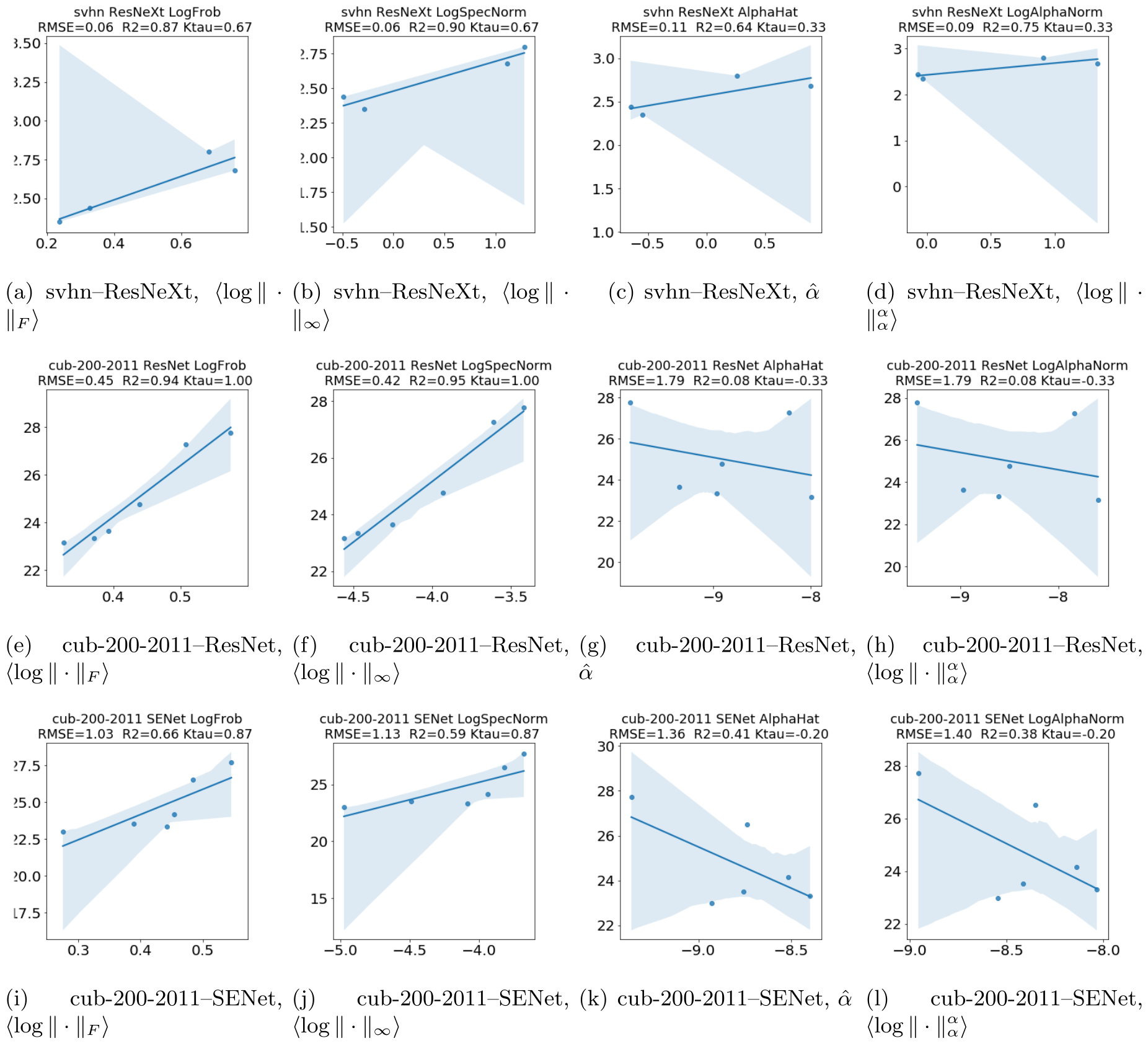
The displayed tables do not fully reconcile with that description: Table 5 includes some four-model series and CUB-200-2011 entries despite the stated exclusions, and Tables 6–8 retain CUB results. They list 27 architecture–dataset groups with four metrics, consistent with 108 regressions rather than 108 individual models. All counts, per-series errors, R² values, and signed Kendall correlations are preserved. They should be read as the supplied analysis record, not silently replaced with a newly inferred selection rule.
| Architecture | of Models | Datasets | ||||
| total | imagenet-1k | cifar-10 | cifar-100 | svhn | cub-200-2011 | |
| EfficientNet | 20 | 20 | 0 | 0 | 0 | 0 |
| ResNet | 48 | 19 | 8 | 8 | 7 | 6 |
| PreResNet | 14 | 14 | 0 | 0 | 0 | 0 |
| VGG/BN-VGG | 12 | 12 | 0 | 0 | 0 | 0 |
| ShuffleNet | 12 | 12 | 0 | 0 | 0 | 0 |
| DLA | 10 | 10 | 0 | 0 | 0 | 0 |
| HRNet | 9 | 9 | 0 | 0 | 0 | 0 |
| DRN-C/DRN-D | 7 | 7 | 0 | 0 | 0 | 0 |
| SqueezeNext/SqNxt | 6 | 6 | 0 | 0 | 0 | 0 |
| ESPNetv2 | 5 | 5 | 0 | 0 | 0 | 0 |
| SqueezeNet/SqueezeResNet | 4 | 4 | 0 | 0 | 0 | 0 |
| IGCV3 | 4 | 4 | 0 | 0 | 0 | 0 |
| ProxylessNAS | 4 | 4 | 0 | 0 | 0 | 0 |
| DIA-ResNet/DIA-PreResNet | 24 | 0 | 8 | 8 | 8 | 0 |
| SENet/SE-ResNet | 20 | 0 | 5 | 5 | 4 | 6 |
| WRN | 8 | 0 | 0 | 4 | 4 | 0 |
| ResNeXt | 4 | 0 | 0 | 0 | 4 | 0 |
| total per dataset | 211 | 126 | 21 | 25 | 27 | 12 |
| Dataset | Model | ||||
| imagenet-1k | EfficientNet | 1.64 | 1.11 | 1.60 | 1.58 |
| imagenet-1k | ResNet | 2.52 | 3.29 | 1.88 | 2.00 |
| imagenet-1k | PreResNet | 2.57 | 3.93 | 1.90 | 1.93 |
| imagenet-1k | VGG | 1.11 | 0.91 | 1.57 | 1.48 |
| imagenet-1k | ShuffleNet | 5.95 | 9.46 | 4.42 | 4.30 |
| imagenet-1k | DLA | 4.79 | 3.02 | 3.94 | 4.06 |
| imagenet-1k | HRNet | 0.64 | 0.77 | 0.36 | 0.36 |
| imagenet-1k | DRN-C | 0.77 | 0.81 | 0.64 | 0.69 |
| imagenet-1k | SqueezeNext | 4.68 | 4.62 | 3.65 | 3.64 |
| imagenet-1k | ESPNetv2 | 3.71 | 3.84 | 1.37 | 1.59 |
| imagenet-1k | SqueezeNet | 0.33 | 0.33 | 0.26 | 0.29 |
| imagenet-1k | IGCV3 | 1.39 | 9.37 | 2.91 | 1.04 |
| imagenet-1k | ProxylessNAS | 0.44 | 0.51 | 0.53 | 0.51 |
| cifar-10 | ResNet | 0.56 | 0.55 | 0.53 | 0.53 |
| cifar-10 | DIA-ResNet | 0.22 | 0.28 | 0.53 | 0.56 |
| cifar-10 | SENet | 0.30 | 0.30 | 0.20 | 0.20 |
| cifar-100 | ResNet | 2.03 | 2.12 | 1.75 | 1.75 |
| cifar-100 | DIA-ResNet | 0.60 | 1.17 | 0.96 | 1.01 |
| cifar-100 | SENet | 0.60 | 0.65 | 0.51 | 0.51 |
| cifar-100 | WRN | 0.37 | 0.44 | 0.26 | 0.25 |
| svhn | ResNet | 0.20 | 0.20 | 0.15 | 0.16 |
| svhn | DIA-ResNet | 0.07 | 0.06 | 0.13 | 0.13 |
| svhn | SENet | 0.04 | 0.07 | 0.05 | 0.05 |
| svhn | WRN | 0.07 | 0.08 | 0.07 | 0.07 |
| svhn | ResNeXt | 0.06 | 0.06 | 0.11 | 0.09 |
| cub-200-2011 | ResNet | 0.45 | 0.42 | 1.79 | 1.79 |
| cub-200-2011 | SENet | 1.03 | 1.13 | 1.36 | 1.40 |
| Dataset | Model | ||||
| imagenet-1k | EfficientNet | 0.65 | 0.84 | 0.67 | 0.67 |
| imagenet-1k | ResNet | 0.77 | 0.61 | 0.87 | 0.86 |
| imagenet-1k | PreResNet | 0.73 | 0.36 | 0.85 | 0.85 |
| imagenet-1k | VGG | 0.63 | 0.75 | 0.27 | 0.35 |
| imagenet-1k | ShuffleNet | 0.63 | 0.06 | 0.80 | 0.81 |
| imagenet-1k | DLA | 0.11 | 0.65 | 0.40 | 0.36 |
| imagenet-1k | HRNet | 0.89 | 0.85 | 0.97 | 0.97 |
| imagenet-1k | DRN-C | 0.81 | 0.79 | 0.87 | 0.85 |
| imagenet-1k | SqueezeNext | 0.05 | 0.07 | 0.42 | 0.43 |
| imagenet-1k | ESPNetv2 | 0.42 | 0.38 | 0.92 | 0.89 |
| imagenet-1k | SqueezeNet | 0.01 | 0.00 | 0.38 | 0.26 |
| imagenet-1k | IGCV3 | 0.98 | 0.12 | 0.92 | 0.99 |
| imagenet-1k | ProxylessNAS | 0.68 | 0.56 | 0.53 | 0.58 |
| cifar-10 | ResNet | 0.58 | 0.59 | 0.62 | 0.61 |
| cifar-10 | DIA-ResNet | 0.96 | 0.93 | 0.74 | 0.71 |
| cifar-10 | SENet | 0.91 | 0.91 | 0.96 | 0.96 |
| cifar-100 | ResNet | 0.61 | 0.58 | 0.71 | 0.71 |
| cifar-100 | DIA-ResNet | 0.96 | 0.85 | 0.90 | 0.89 |
| cifar-100 | SENet | 0.97 | 0.96 | 0.98 | 0.98 |
| cifar-100 | WRN | 0.32 | 0.04 | 0.66 | 0.69 |
| svhn | ResNet | 0.69 | 0.70 | 0.82 | 0.81 |
| svhn | DIA-ResNet | 0.94 | 0.95 | 0.78 | 0.77 |
| svhn | SENet | 0.99 | 0.96 | 0.98 | 0.98 |
| svhn | WRN | 0.13 | 0.10 | 0.20 | 0.21 |
| svhn | ResNeXt | 0.87 | 0.90 | 0.64 | 0.75 |
| cub-200-2011 | ResNet | 0.94 | 0.95 | 0.08 | 0.08 |
| cub-200-2011 | SENet | 0.66 | 0.59 | 0.41 | 0.38 |
| Dataset | Model | ||||
| imagenet-1k | EfficientNet | 0.67 | 0.79 | 0.66 | 0.66 |
| imagenet-1k | ResNet | 0.78 | 0.70 | 0.91 | 0.89 |
| imagenet-1k | PreResNet | 0.65 | 0.54 | 0.87 | 0.87 |
| imagenet-1k | VGG | 0.73 | 0.79 | 0.42 | 0.52 |
| imagenet-1k | ShuffleNet | 0.39 | 0.09 | 0.85 | 0.82 |
| imagenet-1k | DLA | 0.51 | 0.82 | 0.78 | 0.69 |
| imagenet-1k | HRNet | 0.56 | 0.44 | 0.61 | 0.61 |
| imagenet-1k | DRN-C | 0.90 | 0.81 | 0.90 | 0.90 |
| imagenet-1k | SqueezeNext | 0.47 | -0.33 | 0.73 | 0.73 |
| imagenet-1k | ESPNetv2 | 0.00 | 0.80 | 1.00 | 1.00 |
| imagenet-1k | SqueezeNet | 0.33 | 0.00 | 0.67 | 0.67 |
| imagenet-1k | IGCV3 | 1.00 | 0.00 | 1.00 | 1.00 |
| imagenet-1k | ProxylessNAS | 0.33 | 0.33 | 0.33 | 0.33 |
| cifar-10 | ResNet | 0.64 | 0.64 | 0.71 | 0.71 |
| cifar-10 | DIA-ResNet | 0.79 | 0.50 | 0.86 | 0.79 |
| cifar-10 | SENet | 0.74 | 0.95 | 0.95 | 0.95 |
| cifar-100 | ResNet | 0.64 | 0.57 | 0.64 | 0.64 |
| cifar-100 | DIA-ResNet | 0.93 | 0.43 | 0.93 | 0.93 |
| cifar-100 | SENet | 1.00 | 1.00 | 1.00 | 1.00 |
| cifar-100 | WRN | 0.67 | -0.67 | 0.00 | 0.00 |
| svhn | ResNet | 0.81 | 0.71 | 0.81 | 0.81 |
| svhn | DIA-ResNet | 0.86 | 0.86 | 0.57 | 0.57 |
| svhn | SENet | 1.00 | 1.00 | 0.67 | 0.67 |
| svhn | WRN | -0.33 | -0.33 | 0.67 | 0.67 |
| svhn | ResNeXt | 0.67 | 0.67 | 0.33 | 0.33 |
| cub-200-2011 | ResNet | 1.00 | 1.00 | -0.33 | -0.33 |
| cub-200-2011 | SENet | 0.87 | 0.87 | -0.20 | -0.20 |
A.2 Supplementary Tables and Figures
The nine complete twelve-panel figure grids retain all 108 fitted comparisons, their points, lines, confidence bands, and regression statistics. They show that no metric wins uniformly. Power-law metrics improve the displayed PreResNet and several ShuffleNet/SqueezeNext fits, while norm metrics do better in some DIA-ResNet and CUB comparisons; some relationships are weak or have the opposite sign. The confidence bands characterize fitted mean regressions, not a guarantee that 95% of individual model points must lie inside them.
The appendix prose twice calls the rightmost α-norm column a Frobenius norm, although the figure labels identify it as α-norm. It also gives positive 0.33 for SqueezeNext’s spectral-norm Kendall value where Table 8 and the plot show −0.33. The complete figures and tables are retained so these source-label inconsistencies are visible. The evidence supports examining family-specific fits and exceptions rather than relying on the problematic aggregate Table 3.
A.3 Supplementary Discussion: Additional Details on HT-SR Theory
Across nearly 10,000 analyzed layer matrices, the authors report roughly 70–80% of fitted exponents in (2,4) and 10–20% below two, with occasional values near ten or higher. This describes finite fitted spectra under their procedure. It does not establish an asymptotic universality class for every learned matrix or demonstrate that a power law is uniquely preferred over alternative distributions in every case. Very large exponents can signal poor fits, and architecture-specific normalization and extraction remain relevant.