Intuition. Treat training like an engineering learning curve: how much does prediction improve when you buy more parameters, examples or computation? Cross-entropy measures how surprised the model is by real next tokens; lower loss means it assigns them higher probabilities. A power law predicts fractional improvements rather than a fixed gain in accuracy.
Reading the math. N counts model parameters, D counts training tokens and C measures computation. In L(N) ∝ N−α, doubling N multiplies the fitted loss by 2−α, while other bottlenecks are absent. A small α means diminishing returns. Its value is measured from experiments, not a universal constant of language.
Across the tested Transformer language models, cross-entropy loss follows approximate power laws in model size, data, and training compute. The paper combines these fits to estimate efficient training allocations and argues for larger models stopped before convergence. These are empirical laws for the studied data, models, and optimization regime; the paper itself identifies extrapolation limits and incompatible far-future predictions.
1 Introduction
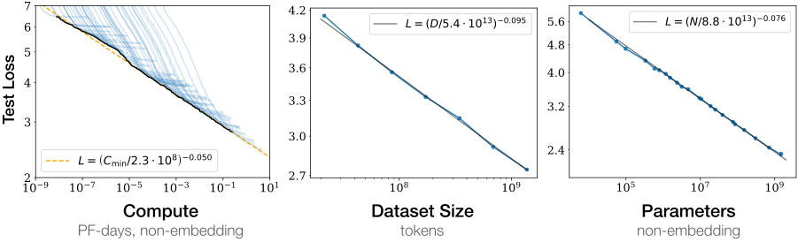
The study measures predictive loss rather than an omnibus intelligence score. It varies architecture, model size, available text, and training budget over wide ranges, seeking equations that can forecast held-out language-model performance. Figure 1 summarizes the separately model-, data-, and compute-limited regimes.
Figure 1:Language modeling performance improves smoothly as we increase the model size, datasetset size, and amount of compute111
Here we display predicted compute when using a sufficiently small batch size. See Figure13 for comparison to the purely empirical data. used for training. For optimal performance all three factors must be scaled up in tandem. Empirical performance has a power-law relationship with each individual factor when not bottlenecked by the other two.
1.1 Summary
The following findings summarize the measured trends before the methods, fits, and caveats are developed.
Performance depends strongly on scale, weakly on model shape:
Non-embedding parameter count, data size, and training compute explain much more variation than moderate changes in Transformer depth or width at fixed size.
Smooth power laws:
Approximate power laws fit broad observed ranges when the other resources are sufficient. Their continuation to arbitrarily low loss is impossible because language has residual uncertainty.
Universality of overfitting:
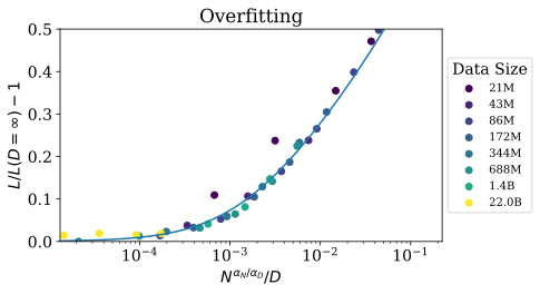
Jointly increasing model and dataset size controls overfitting. Under the fitted finite-data relationship, preserving the relative penalty requires dataset size to grow approximately as parameter count to the power 0.74.
Universality of training:
After early training transients, learning curves admit a common parameterized form. Extrapolation is useful within that regime, not a guarantee about initial optimization or very distant scales.
Transfer improves with test performance:
On the tested alternative text distributions, loss largely tracks in-distribution loss with an offset. The evidence concerns predictive text likelihood, not every downstream transfer task.
Sample efficiency:
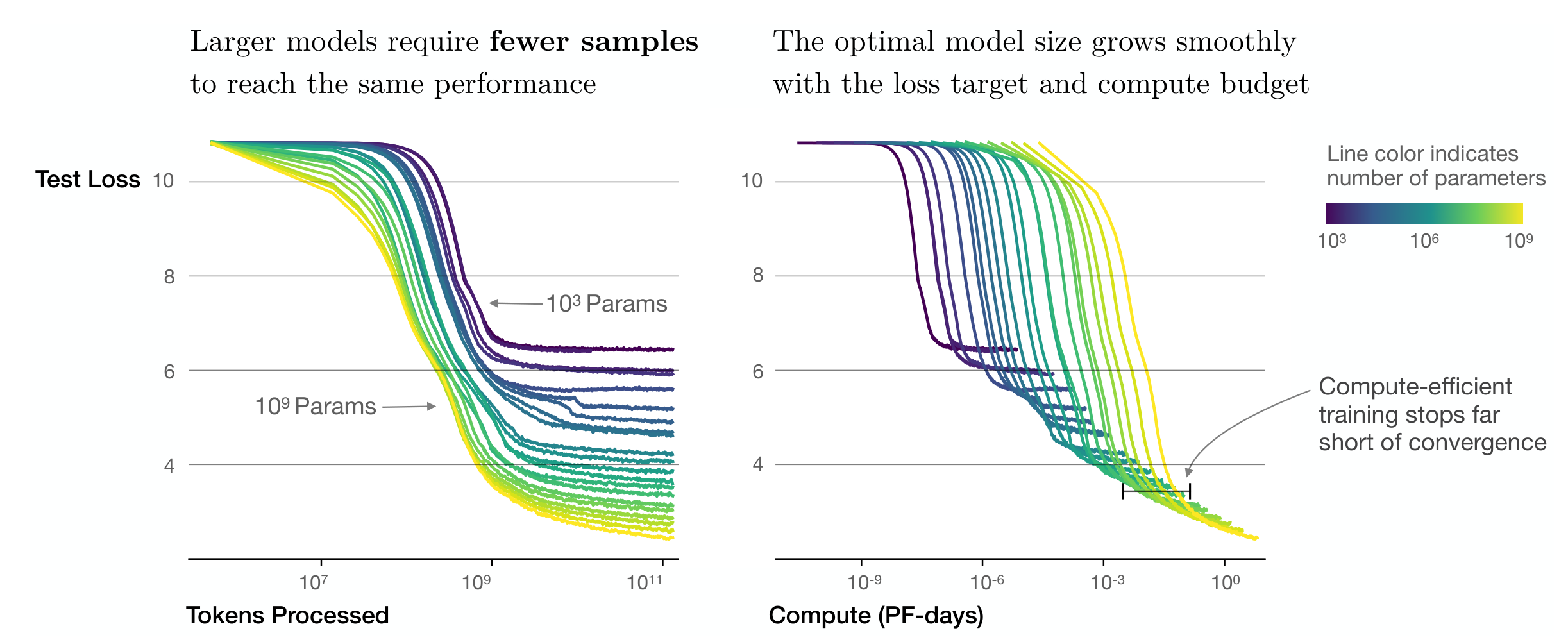
Larger models can reach a fixed loss with fewer data examples and fewer update steps. This sample efficiency does not mean each step is cheaper; the later analysis trades those costs against model size.
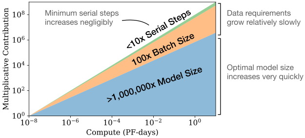
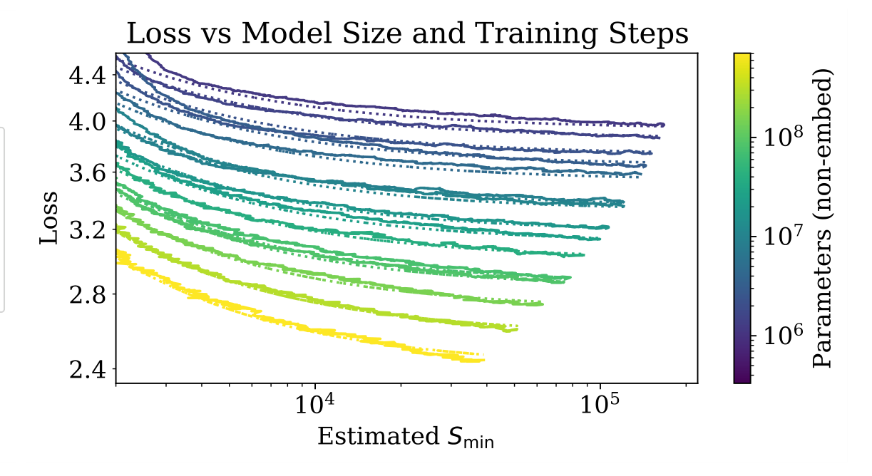
Figure 2:We show a series of language model training runs, with models ranging in size from to parameters (excluding embeddings).Figure 3:As more compute becomes available, we can choose how much to allocate towards training larger models, using larger batches, and training for more steps. We illustrate this for a billion-fold increase in compute. For optimally compute-efficient training, most of the increase should go towards increased model size. A relatively small increase in data is needed to avoid reuse. Of the increase in data, most can be used to increase parallelism through larger batch sizes, with only a very small increase in serial training time required.
Convergence is inefficient:
Within the paper’s fitted training regime, compute-efficient runs use larger models and stop before full convergence. The reported data-growth exponent is a conclusion of this historical fit, not a universal training prescription.
Optimal batch size:
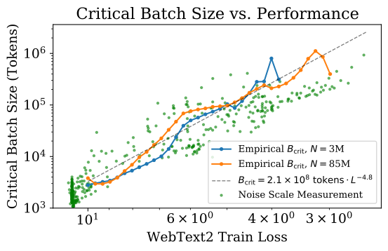
Critical batch size is related primarily to achieved loss and gradient noise scale. Beyond it, extra parallel examples buy diminishing reductions in update count.
1.2 Summary of Scaling Laws
Separate fits describe loss as a function of parameters, data, and batch-adjusted compute. Joint models then combine finite-data penalties or unfinished optimization with the parameter-limited loss. The equations retain their original constants and exponents; different fitting subsets yield slightly different values, and tokenization-dependent constants have no universal meaning.
Equations 1.1–1.4
(1.1)
(1.2)
(1.3)
(1.4)
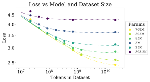
Figure 4:Left: The early-stopped test loss varies predictably with the dataset size and model size according to Equation (1.5).
Right: After an initial transient period, learning curves for all model sizes can be fit with Equation (1.6), which is parameterized in terms of, the number of steps when training at large batch size (details in Section5.1).
Equations 1.5–1.8
(1.5)
(1.6)
(1.7)
(1.8)
1.3 Notation
Loss is measured in nats per token. N excludes token and positional embeddings; D counts tokens; B is batch size in tokens; S counts updates. Training compute is approximated by 6NBS. The adjusted quantities C_min and S_min describe different limiting batch regimes and should not be confused with directly observed FLOPs or steps.
2 Background and Methods
Decoder-only Transformers predict tokens in 1,024-token contexts using WebText2 and a 50,257-token byte-pair vocabulary. Held-out cross-entropy is the main metric. LSTMs and parameter-sharing Universal Transformers provide architectural comparisons.
2.1 Parameter and Compute Scaling of Transformers
Parameter and FLOP estimates omit embeddings, biases, nonlinearities, and smaller terms. The approximation of six non-embedding parameter operations per training token is appropriate when context-dependent attention work is relatively small. Very long contexts can violate that assumption.
Table 1:Parameter counts and compute (forward pass) estimates for a Transformer model. Sub-leading terms such as nonlinearities, biases, and layer normalization are omitted.
Equations 2.1–2.2
(2.1)
(2.2)
2.2 Training Procedures
Most runs use Adam, 250,000 updates, and batches of 512 sequences, with warmup and cosine decay. Models above one billion parameters use Adafactor because of memory constraints. Learning schedules are studied separately, but optimizer and hyperparameter coverage remain limited.
2.3 Datasets
WebText2 extends the Reddit-linked WebText collection through October 2018, producing 20.3 million documents and about 22.9 billion tokens. The study holds out 660 million tokens and evaluates additional book, web, and Wikipedia distributions. Reddit-link selection is a sampling heuristic, not representative coverage of all language.
3 Empirical Results and Basic Power Laws
Experiments vary non-embedding model sizes from 768 to 1.5 billion parameters, datasets from 22 million to 23 billion tokens, model shape, context, and batch size. The fitted domain is defined by these experiments.
3.1 Approximate Transformer Shape and Hyperparameter Independence
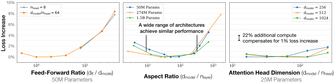
At fixed non-embedding parameter count, broad but non-extreme changes in depth, width, heads, and feed-forward dimension alter loss by only a few percent. This is approximate architectural insensitivity within the investigated family, not equivalence between arbitrary architectures.
Figure 5:Performance depends very mildly on model shape when the total number of non-embedding parameters is held fixed. The loss varies only a few percent over a wide range of shapes. Small differences in parameter counts are compensated for by using the fit to as a baseline. Aspect ratio in particular can vary by a factor of 40 while only slightly impacting performance; an reaches a loss within 3% of the model used in[RWC+19].
3.2 Performance with Non-Embedding Parameter Count N
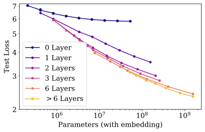
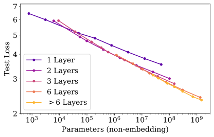
Excluding embedding parameters aligns models of different shapes into a cleaner loss–size trend. One-layer models and extreme aspect ratios deviate. Near-converged training on the full corpus supplies the parameter-scaling fit; incomplete convergence must be distinguished from insufficient capacity.
Figure 6:Left: When we include embedding parameters, performance appears to depend strongly on the number of layers in addition to the number of parameters.
Right: When we exclude embedding parameters, the performance of models with different depths converge to a single trend. Only models with fewer than 2 layers or with extreme depth-to-width ratios deviate significantly from the trend.Equation 3.1
(3.1)
3.2.1 Comparing to LSTMs and Universal Transformers
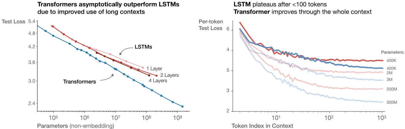
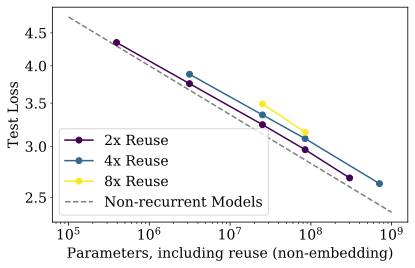
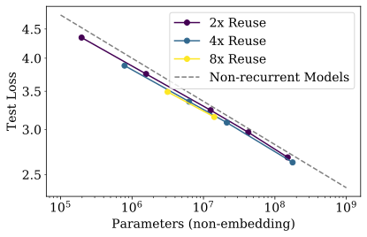
LSTMs compare well on early context tokens but benefit less from later context than Transformers. Universal Transformers reuse parameters and gain slightly per parameter, while losing slightly per unit of compute. The appropriate comparison changes with the resource being constrained.
Figure 7:
3.2.2 Generalization Among Data Distributions
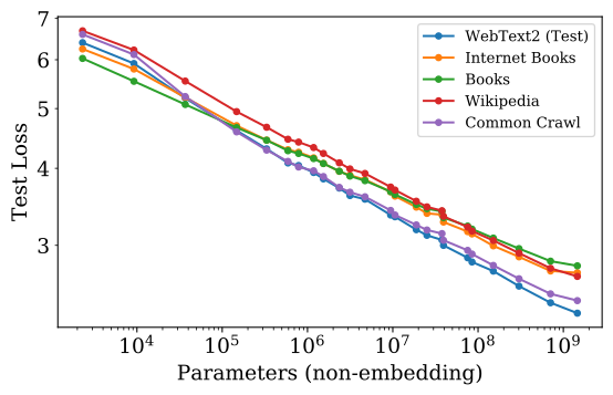
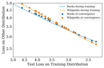
Other text distributions improve roughly in parallel with WebText2 loss, across both model sizes and training progress. In the measured settings, held-out training-distribution performance is more predictive of this transfer than depth or proximity to convergence.
Figure 8:Left: Generalization performance to other data distributions improves smoothly with model size, with only a small and very slowly growing offset from the WebText2 training distribution.
Right: Generalization performance depends only on training distribution performance, and not on the phase of training. We compare generalization of converged models (points) to that of a single large model (dashed curves) as it trains.
3.3 Performance with Dataset Size and Compute
Data-limited fits use fixed dataset subsets with early stopping. Compute-limited comparisons search model training curves at equal estimated budgets; the initial fixed-batch analysis is subsequently adjusted for batch inefficiency. These are distinct experimental regimes rather than interchangeable curves.
Equations 3.2–3.3
(3.2)
(3.3)
4 Charting the Infinite Data Limit and Overfitting
The joint model-and-data fit estimates how finite data limits otherwise larger models. Early stopping and fixed regularization are part of the setup.
4.1 Proposed L ( N , D ) Equation
The proposed formula matches separate infinite-data and infinite-model limits and permits loss rescaling under tokenization changes. Its analytic expansion in inverse dataset size is more speculative. Empirical fit quality is the principal justification; it is not derived as a general theorem about neural networks.
Figure 9:
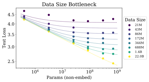
The early-stopped test loss depends predictably on the dataset size and model size according to Equation (1.5).
Left:
For large, performance is a straight power law in. For a smaller fixed, performance stops improving as increases and the model begins to overfit. (The reverse is also true, see Figure4.)
Right: The extent of overfitting depends predominantly on the ratio, as predicted in equation (4.3). The line is our fit to that equation.
Equation 4.1
(4.1)
4.2 Results
The formula fits most tested sizes but is weaker on the smallest dataset, where an epoch is only forty updates. A practical overfitting threshold is inferred from approximately 0.02 loss variation between seeds. Dropout was fixed rather than optimized across all dataset and model sizes, limiting universality.
Parameter
Value
Table 2:Fits to
Equations 4.2–4.4
(4.2)
(4.3)
(4.4)
5 Scaling Laws with Model Size and Training Time
A batch-adjusted training-step variable helps compare learning curves that were not trained at their own optimal batch sizes.
5.1 Adjustment for Training at B crit ( L )
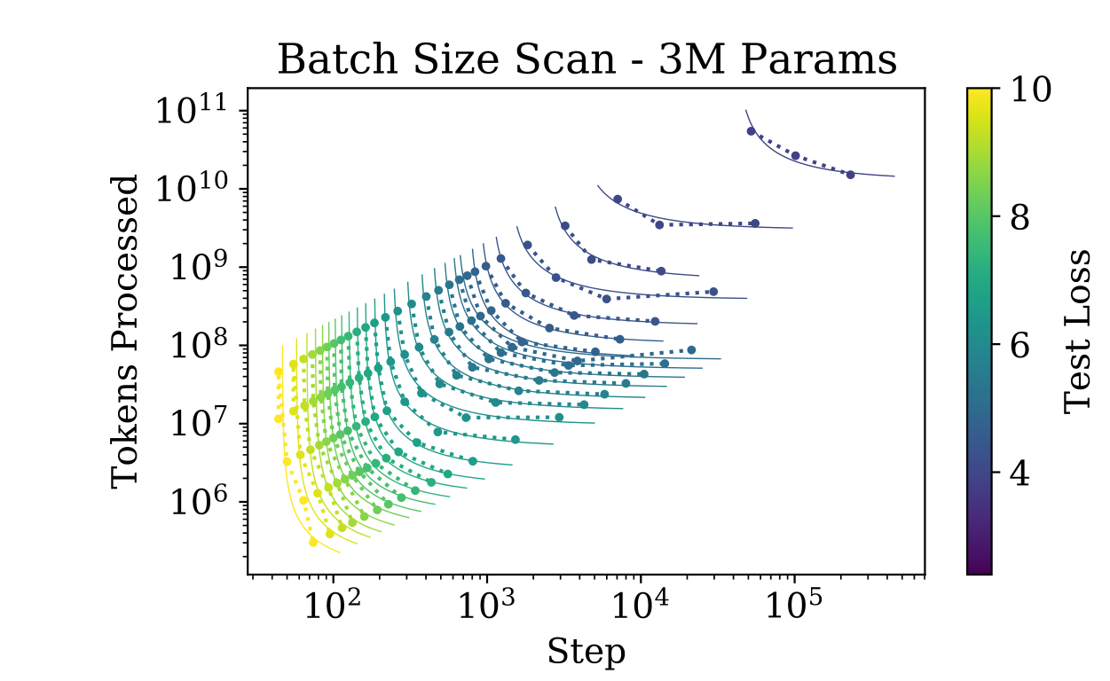
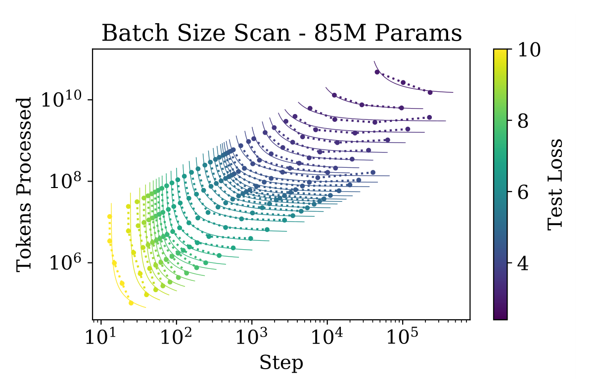
Small batches minimize examples and compute needed for a target loss; very large batches minimize serial updates. The critical batch lies near the tradeoff. The paper fits its dependence on loss and uses that empirical relation to estimate minimum-compute and minimum-step curves from fixed-batch runs.
Figure 10:The critical batch size follows a power law in the loss as performance increase, and does not depend directly on the model size. We find that the critical batch size approximately doubles for every decrease in loss. is measured empirically from the data shown in Figure18, but it is also roughly predicted by the gradient noise scale, as in[MKAT18].Equations 5.1–5.5
(5.1)
(5.2)
(5.3)
(5.4)
(5.5)
5.2 Results for L ( N , S min ) and Performance with Model Size and Compute
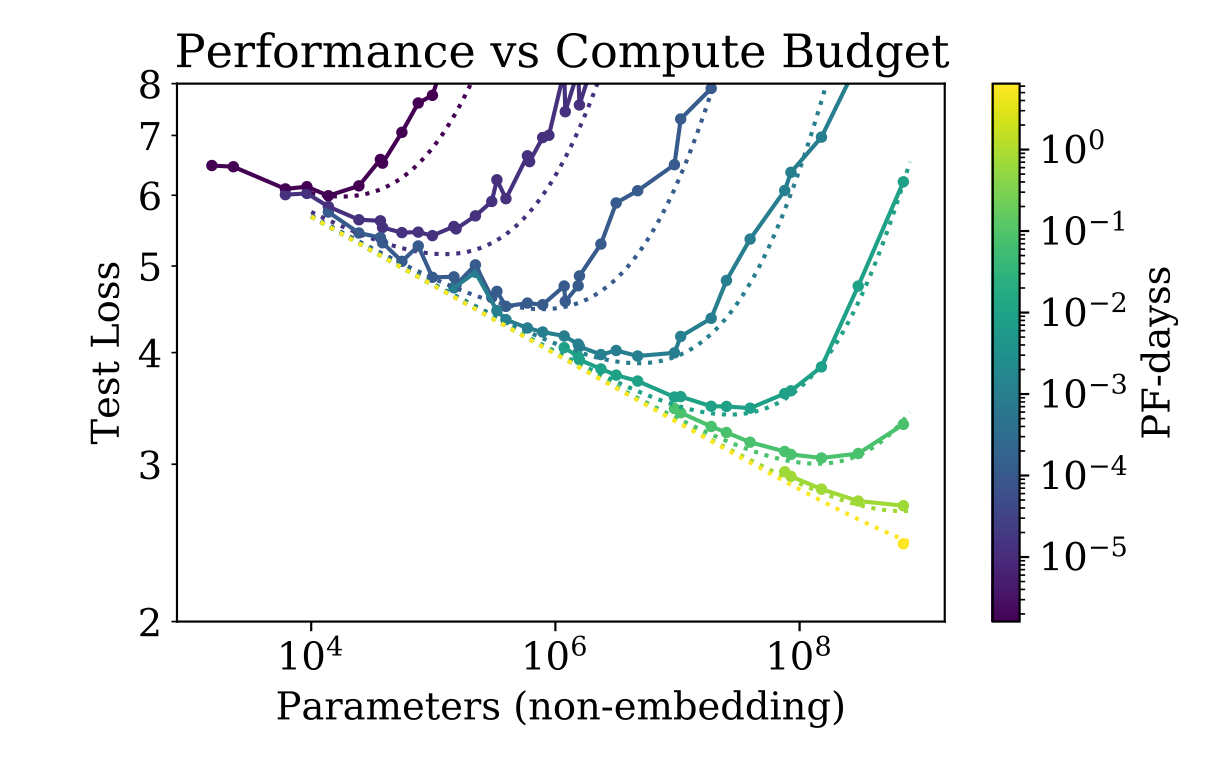
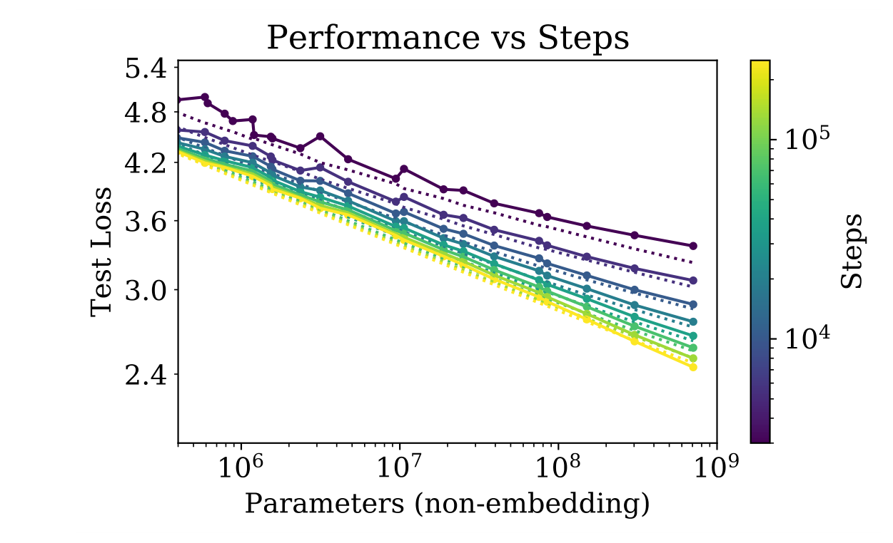
After warmup, loss is fitted as a parameter-limited term plus a decaying optimization term. At fixed compute, making the model larger eventually leaves too few updates, yielding an intermediate best size. Fit deviations at early steps are expected because the power-law regime has not yet begun.
Figure 11:
When we hold either total compute or number of training steps fixed, performance follows from Equation (5.6). Each value of compute budget has an associated optimal model size that maximizes performance. Mediocre fits at small are unsurprising, as the power-law equation for the learning curves breaks down very early in training.Equation 5.6
(5.6)
Parameter
Value
Table 3:Fits to
5.3 Lower Bound on Early Stopping Step
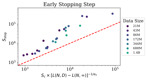
Comparing finite-data and infinite-data loss suggests a lower bound on when early stopping should occur. The derivation treats their curves as similar until overfitting matters; the actual finite-data curve can improve more slowly. It is therefore a bound and rough estimate, not an exact stopping rule.
Equation 5.7
(5.7)
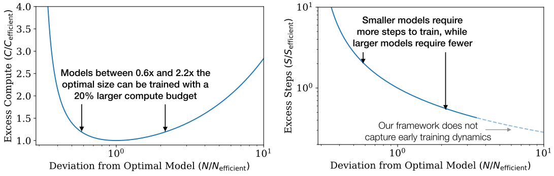
Figure 12:Left: Given a fixed compute budget, a particular model size is optimal, though somewhat larger or smaller models can be trained with minimal additional compute.Right: Models larger than the compute-efficient size require fewer steps to train, allowing for potentially faster training if sufficient additional parallelism is possible. Note that this equation should not be trusted for very large models, as it is only valid in the power-law region of the learning curve, after initial transient effects.
6 Optimal Allocation of the Compute Budget
The compute frontier corrects the fixed-batch experiments using measured critical-batch behavior, then balances parameter count against data processed and serial training time. Adjusted estimates should be distinguished from direct runs at every predicted optimal setting.
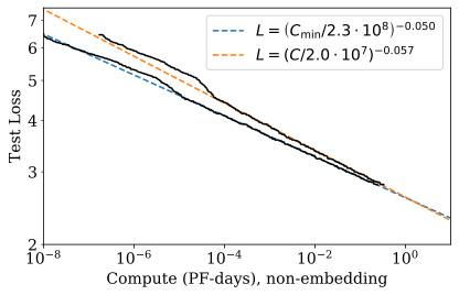
Figure 13:
When adjusting performance to simulate training far below the critical batch size, we find a somewhat altered power law for when compared with the fully empirical results. The conspicuous lump at PF-days marks the transition from 1-layer to 2-layer networks; we exclude 1-layer networks in the power-law fits. It is the trend that we expect to provide a reliable extrapolation for larger compute.
6.1 Optimal Performance and Allocations
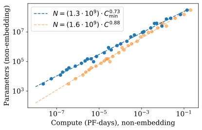
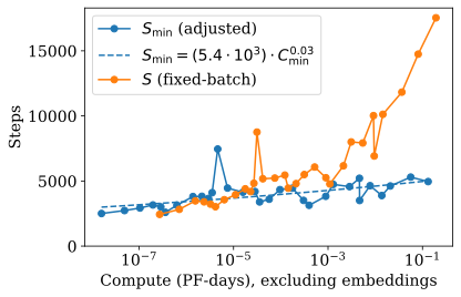
The empirical frontier gives approximate exponents 0.73 for model size, 0.24 for batch size, and 0.03 for minimum steps as compute grows. Thus most extra budget goes into larger models within this fit. The tiny step exponent is uncertain enough to be compatible with little or no growth.
Equations 6.1–6.2
(6.1)
(6.2)
Figure 14:Left: Each value of the compute budget has an associated optimal model size. Optimal model size grows very rapidly with, increasing by 5x for each 10x increase in compute. The number of data examples processed makes up the remainder of the increase, growing relatively modestly by only 2x.
Right: The batch-adjusted number of optimization steps also grows very slowly, if at all, meaning that most of the growth in data examples processed can be used for increased batch sizes.
6.2 Predictions from L ( N , S min )
Minimizing the fitted learning-curve equation predicts loss and model-size exponents close to those measured on the adjusted frontier. This internal agreement supports the framework over its experimental range; it does not independently verify arbitrary extrapolations.
Equations 6.3–6.5
(6.3)
(6.4)
(6.5)
6.3 Contradictions and a Conjecture
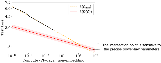
Far beyond the measured regime, the predicted data requirement conflicts with the predicted compute-efficient loss. At least one relation must change before their intersection. The suggested trillion-parameter/trillion-token scale and natural-language entropy interpretation are explicitly uncertain conjectures, sensitive to fitted exponents, rather than established limits.
Figure 15:Far beyond the model sizes we study empirically, we find a contradiction between our equations for and due to the slow growth of data needed for compute-efficient training. The intersection marks the point before which we expect our predictions to break down. The location of this point is highly sensitive to the precise exponents from our power-law fits.Equations 6.6–6.8
(6.6)
(6.7)
(6.8)
7 Related Work
The paper connects its results to prior learning curves, dataset scaling, efficient architectures, overparameterization, and noisy optimization models. Earlier studies found different data–model relationships, reinforcing that training setup and the quantity held fixed matter.
8 Discussion
The main value is a predictive empirical framework for allocation within a studied regime. The authors leave open which trends generalize to other modalities and whether lower text loss translates into meaningful task improvements. Diminishing returns, hardware parallelism, and omitted inference costs also matter when applying the findings.
Acknowledgements
The authors acknowledge colleagues for discussions and comments on drafts.
Appendix A Summary of Power Laws
The six tables collect the fitted regimes, constants, and compute-efficient allocations. They retain which variables are fixed, unlimited, or optimized; constants differ among separate and joint fits and depend on tokenization.
Appendix B Empirical Model of Compute-Efficient Frontier
This appendix derives an efficient frontier from the fitted learning curve and batch-size relation. Its notation suppresses the batch-adjustment label, so symbols should be interpreted with that convention.
B.1 Defining Equations
Substitute compute divided by model size and batch size for the update count, then differentiate loss with respect to model size at fixed compute. The resulting optimum balances the capacity-limited and unfinished-training terms. The retained equations show the assumptions and algebra.
Equations B.1–B.4
(B.1)
(B.2)
(B.3)
(B.4)
B.2 Efficient Training
The fitted optimum stops at a loss about 10% above the same model’s asymptotic loss. Eliminating either model size or loss yields the predicted power laws for efficient compute, parameters, and updates.
Equations B.5–B.10
(B.5)
(B.6)
(B.7)
(B.8)
(B.9)
(B.10)
B.3 Comparison to Inefficient
Against a model trained to within 2% of its converged loss, the fitted 10%-gap strategy uses about 2.7 times as many parameters, 7.7 times fewer updates, and 65% less training compute at equal target loss. These are consequences of the empirical model, not measurements guaranteed for every workload.
Equations B.11–B.14
(B.11)
(B.12)
(B.13)
(B.14)
B.4 Suboptimal Model Sizes
The efficient optimum is fairly broad: sizes from about 0.6 to 2.2 times optimal need only around 20% extra training compute in the fit. Smaller models may reduce inference costs; larger ones may shorten serial training if parallel hardware is available. The paper’s unresolved figure placeholders refer to this tradeoff, illustrated in Figure 12.
Equations B.15–B.17
(B.15)
(B.16)
(B.17)
Appendix C Caveats
The authors lack a complete theory and caution against extrapolating critical batch size, small-data behavior, or long-context compute estimates. Regularization, augmentation, initialization, momentum, and short-run learning rates were not comprehensively tuned. These limitations directly affect the allocation exponents and are essential to interpreting the headline recommendation.
Appendix D Supplemental Figures
The supplemental figures retain training-versus-test behavior and parameter-sharing comparisons before the more detailed diagnostics below.
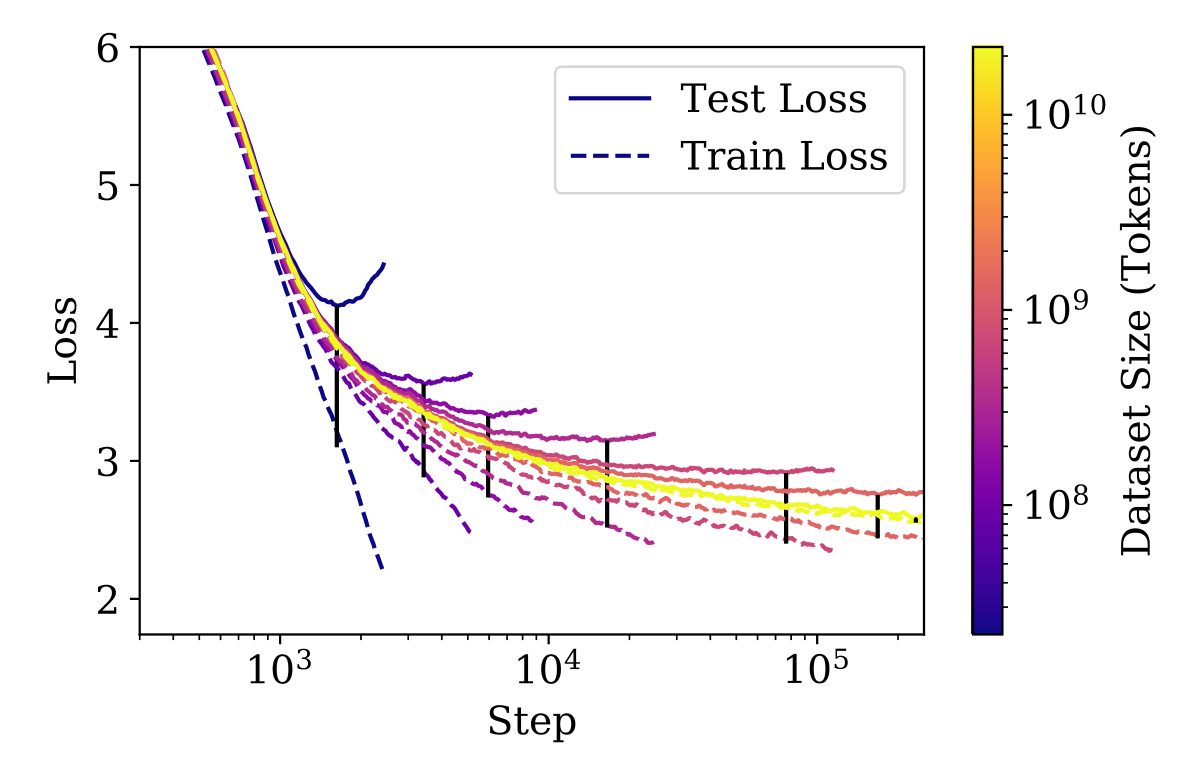
Figure 16:Left: We characterize the step on which early stopping occurs, as a function of the extent of overfitting. The red line indicates a lower bound for early stopping that is derived in Section5.3.Right: We display train and test loss for a series of 300M parameter models trained on different sized dataset sub-samples. The test loss typically follows that of a run done with unrestricted data until diverging. Note that the degree of overfitting (as compared to the infinite data limit) is significantly overestimated by (denoted by a black bar for each run).
Figure 17:We compare recurrent Transformers[DGV+18], which re-use parameters, to standard Transformers. Recurrent Transformers perform slightly better when comparing models with equal parameter count, but slightly worse when accounting for reuse and comparing per FLOP.
D.1 Early Stopping and Test vs Train
The early-stopping plot compares the derived lower bound with measured stopping times. The ordinary train–test gap can overstate the finite-data penalty relative to a model trained on effectively unlimited data.
D.2 Universal Transformers
Parameter reuse modestly improves loss per parameter but modestly worsens loss per FLOP in the tested Universal Transformers. Parameter efficiency and compute efficiency are different objectives.
D.3 Batch Size
Batch-size sweeps at fixed target losses supply the fitted critical-batch measurements used in the main allocation analysis. The two model sizes provide a check on the proposed loss-based dependence.
Figure 18:These figures demonstrate fits to Equation (5.1) for a large number of values of the loss, and for two different Transformer model sizes. These fits were used to measure for Figure10.
D.4 Sample Efficiency vs Model Size
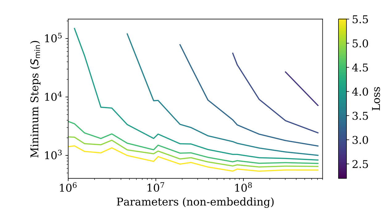
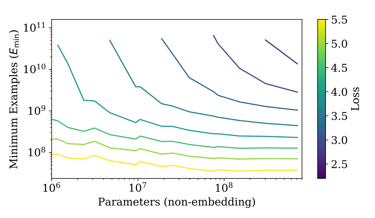
At a fixed target loss, larger models need fewer serial updates and data examples. The curves illustrate substantial sample-efficiency gains while leaving the higher cost per model evaluation visible in the separate compute analysis.
Figure 19:The number of minimum serial steps needed to reach any fixed value of the test loss decreases precipitously with model size. Sample efficiency (show here for training far below the critical batch size) improves greatly as well, improving by a factor of almost 100 when comparing the smallest possible model to a very large one.
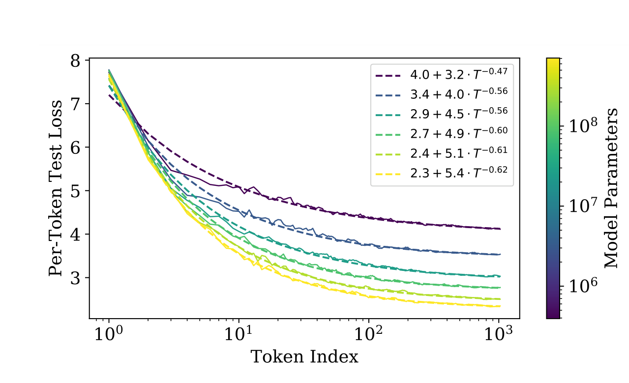
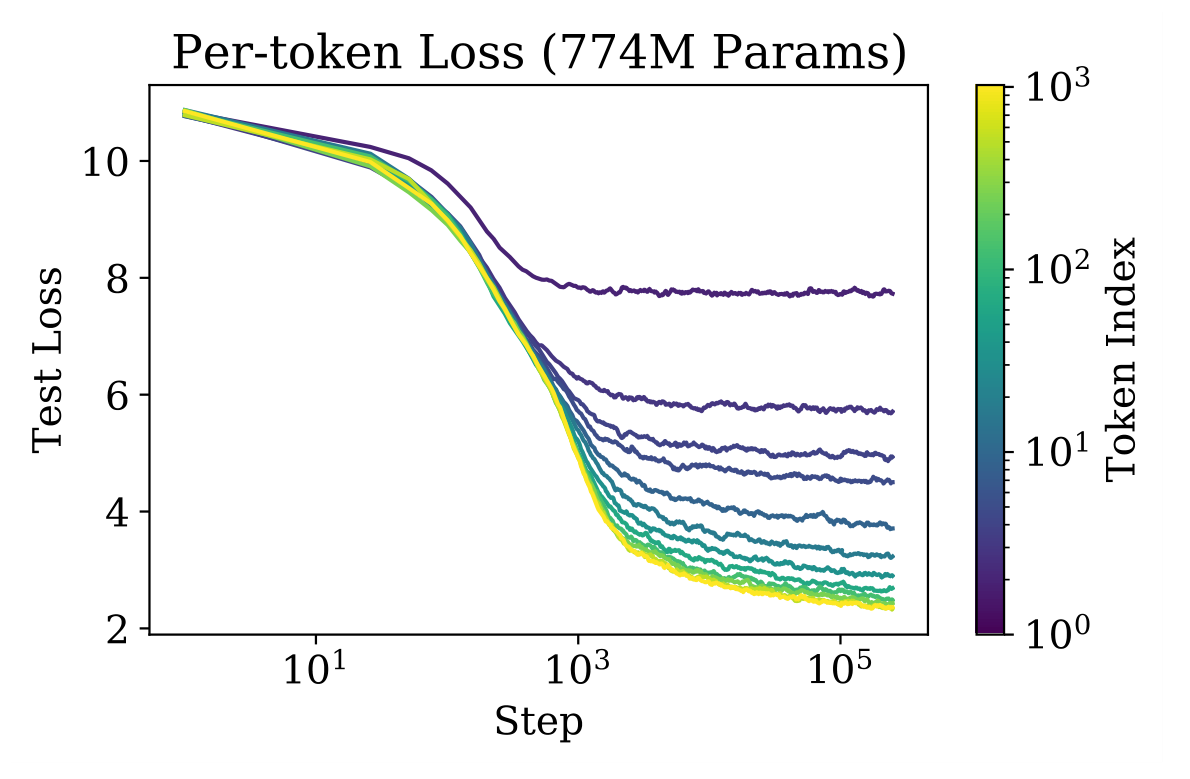
Figure 20: This figure provides information about the performance per token as a function of model size and training time.Left: Loss per token as a function of its position in the 1024-token context. Loss scales predictably as a power-law in.Right: Test loss per token as a function of training step.
D.5 Context Dependence
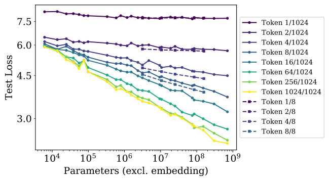
Larger models improve prediction across context positions and exploit patterns with less preceding text. During training, short-range structure appears before longer-range dependencies. Models trained with eight-token contexts can outperform longer-context models on early tokens, showing that average loss reflects a capacity-allocation tradeoff.
Figure 21:In addition to the averaged loss, individual tokens within the 1024-token context also improve smoothly as model size increases. Training runs with shorter context (dashed lines) perform better on early tokens, since they can allocate all of their capacity to them.
Figure 22:
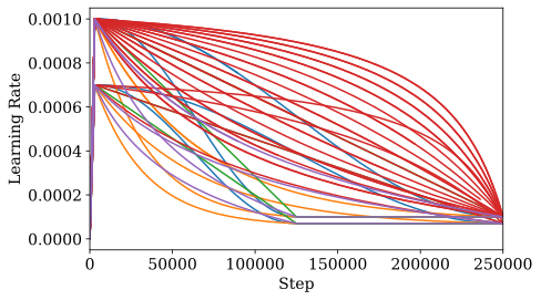
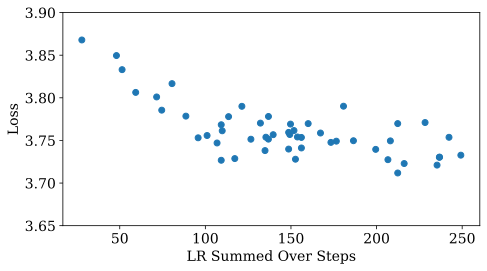
We test a variety of learning rate schedules including cosine decay, linear decay, as well as other faster/slower decays schedules on a 3 million parameter model, shown on the left.
For these experiments we do not decay to zero, since we find that this tends to give a fixed improvement close to the end of training.
We find that, as long as the learning rate is not too small and does not decay too quickly, performance does not depend strongly on learning rate.
Run-to-run variation is at the level of 0.05 in the loss, so averaging multiple runs is necessary to validate performance changes smaller than this level.
D.6 Learning Rate Schedules and Error Analysis
Several schedules yield similar final losses when warmup, sufficient learning, and late decay are present. Random-seed variation limits small comparisons. A practical learning-rate formula decreases with model size but is explicitly invalid beyond its fitted range.
Equation D.1
(D.1)
D.7 Fit Details and Power Law Quality
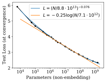
Power laws fit the observed trends better than the tested logarithmic alternatives. Fits exclude one-layer models and, for parameter scaling, very large models that have not converged. Those exclusions define the fitting procedure rather than exceptions hidden from the reader.
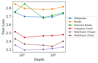
Figure 23:The trend for performance as a function of parameter count,, is fit better by a power law than by other functions such as a logarithm at a qualitative level.Figure 24:We show evaluations on a series of datasets for models with approximately 1.5 Billion parameters. We observe no effect of depth on generalization; generalization performance depends primarily on training distribution performance. The 12-layer model overfit the Internet Books dataset and we show the early-stopped performance; we have not seen this surprising result in other experiments.
D.8 Generalization and Architecture
At roughly fixed parameter count, depth does not materially alter cross-distribution performance after conditioning on in-distribution loss. One Internet Books overfitting case is noted as unusual. The paper’s concluding figure and table indexes contain no additional experimental material.
50 references
[ACDE12]
Eduardo G Altmann, Giampaolo Cristadoro, and Mirko Degli Esposti.
On the origin of long-range correlations in texts.
Proceedings of the National Academy of Sciences,
109(29):11582–11587, 2012.
[BB01]
Michele Banko and Eric Brill.
Scaling to very very large corpora for natural language
disambiguation.
InProceedings of the 39th annual meeting on association for
computational linguistics, pages 26–33. Association for Computational
Linguistics, 2001.
[BHMM18]
Mikhail Belkin, Daniel Hsu, Siyuan Ma, and Soumik Mandal.
Reconciling modern machine learning and the bias-variance trade-off.
arXiv, 2018,
1812.11118.
[DCLT18]
Jacob Devlin, Ming-Wei Chang, Kenton Lee, and Kristina Toutanova.
Bert: Pre-training of deep bidirectional transformers for language
understanding, 2018,
arXiv:1810.04805.
[GJS+19]
Mario Geiger, Arthur Jacot, Stefano Spigler, Franck Gabriel, Levent Sagun,
Stéphane d’Ascoli, Giulio Biroli, Clément Hongler, and Matthieu
Wyart.
Scaling description of generalization with number of parameters in
deep learning.
arXiv, 2019,
1901.01608.
[GKX19]
Behrooz Ghorbani, Shankar Krishnan, and Ying Xiao.
An investigation into neural net optimization via hessian eigenvalue
density.
CoRR, abs/1901.10159, 2019,
1901.10159.
URLhttp://arxiv.org/abs/1901.10159.
[HAD19]
Joel Hestness, Newsha Ardalani, and Gregory Diamos.
Beyond human-level accuracy: Computational challenges in deep
learning.
InProceedings of the 24th Symposium on Principles and Practice
of Parallel Programming, PPoPP ’19, pages 1–14, New York, NY, USA, 2019.
ACM.
doi:10.1145/3293883.3295710.
[HNA+17]
Joel Hestness, Sharan Narang, Newsha Ardalani, Gregory Diamos, Heewoo Jun,
Hassan Kianinejad, Md. Mostofa Ali Patwary, Yang Yang, and Yanqi Zhou.
Deep learning scaling is predictable, empirically, 2017,
1712.00409.
[JGH18]
Arthur Jacot, Franck Gabriel, and Clément Hongler.
Neural tangent kernel: Convergence and generalization in neural
networks.
InAdvances in neural information processing systems, pages
8571–8580, 2018.
[KSH12]
Alex Krizhevsky, Ilya Sutskever, and Geoffrey E. Hinton.
Imagenet classification with deep convolutional neural networks.
InProceedings of the 25th International Conference on Neural
Information Processing Systems - Volume 1, NIPS’12, pages 1097–1105, USA,
2012. Curran Associates Inc.
URLhttp://dl.acm.org/citation.cfm?id=2999134.2999257.
[LCG+19]
Zhenzhong Lan, Mingda Chen, Sebastian Goodman, Kevin Gimpel, Piyush Sharma, and
Radu Soricut.
Albert: A lite bert for self-supervised learning of language
representations, 2019,1909.11942.
[LOG+19]
Yinhan Liu, Myle Ott, Naman Goyal, Jingfei Du, Mandar Joshi, Danqi Chen, Omer
Levy, Mike Lewis, Luke Zettlemoyer, and Veselin Stoyanov.
Roberta: A robustly optimized BERT pretraining approach.
CoRR, abs/1907.11692, 2019,
1907.11692.
URLhttp://arxiv.org/abs/1907.11692.
[LSP+18]
Peter J. Liu, Mohammad Saleh, Etienne Pot, Ben Goodrich, Ryan Sepassi, Lukasz
Kaiser, and Noam Shazeer.
Generating wikipedia by summarizing long sequences.
arXiv:1801.10198 [cs], 2018,
1801.10198.
URLhttp://arxiv.org/abs/1801.10198.
[LXS+19]
Jaehoon Lee, Lechao Xiao, Samuel S. Schoenholz, Yasaman Bahri, Roman Novak,
Jascha Sohl-Dickstein, and Jeffrey Pennington.
Wide neural networks of any depth evolve as linear models under
gradient descent, 2019,
arXiv:1902.06720.
[RRBS19a]
Jonathan S. Rosenfeld, Amir Rosenfeld, Yonatan Belinkov, and Nir Shavit.
A constructive prediction of the generalization error across scales,
2019,1909.12673.
[RRBS19b]
Jonathan S. Rosenfeld, Amir Rosenfeld, Yonatan Belinkov, and Nir Shavit.
A constructive prediction of the generalization error across scales,
2019,arXiv:1909.12673.
[RSR+19]
Colin Raffel, Noam Shazeer, Adam Roberts, Katherine Lee, Sharan Narang, Michael
Matena, Yanqi Zhou, Wei Li, and Peter J. Liu.
Exploring the limits of transfer learning with a unified text-to-text
transformer, 2019,
arXiv:1910.10683.
[RWC+19]
Alec Radford, Jeff Wu, Rewon Child, David Luan, Dario Amodei, and Ilya
Sutskever.
Language models are unsupervised multitask learners.
openai.com, 2019.
[SLA+18]
Christopher J. Shallue, Jaehoon Lee, Joe Antognini, Jascha Sohl-Dickstein, Roy
Frostig, and George E. Dahl.
Measuring the effects of data parallelism on neural network training,
2018,arXiv:1811.03600.
[TL19]
Mingxing Tan and Quoc V. Le.
Efficientnet: Rethinking model scaling for convolutional neural
networks.
CoRR, abs/1905.11946, 2019,
1905.11946.
URLhttp://arxiv.org/abs/1905.11946.
[VSP+17]
Ashish Vaswani, Noam Shazeer, Niki Parmar, Jakob Uszkoreit, Llion Jones,
Aidan N Gomez, Ł ukasz Kaiser, and Illia Polosukhin.
Attention is all you need.
In I. Guyon, U. V. Luxburg, S. Bengio, H. Wallach, R. Fergus,
S. Vishwanathan, and R. Garnett, editors,Advances in Neural Information
Processing Systems 30, pages 5998–6008. Curran Associates, Inc., 2017.
URLhttp://papers.nips.cc/paper/7181-attention-is-all-you-need.pdf.
[VWB16]
Andreas Veit, Michael Wilber, and Serge Belongie.
Residual networks behave like ensembles of relatively shallow
networks, 2016,
arXiv:1605.06431.
[WPN+19]
Alex Wang, Yada Pruksachatkun, Nikita Nangia, Amanpreet Singh, Julian Michael,
Felix Hill, Omer Levy, and Samuel R. Bowman.
Superglue: A stickier benchmark for general-purpose language
understanding systems, 2019,
1905.00537.
[WRH17]
Yu-Xiong Wang, Deva Ramanan, and Martial Hebert.
Growing a brain: Fine-tuning by increasing model capacity.
2017 IEEE Conference on Computer Vision and Pattern Recognition
(CVPR), Jul 2017.
doi:10.1109/cvpr.2017.323.
[YDY+19]
Zhilin Yang, Zihang Dai, Yiming Yang, Jaime Carbonell, Ruslan Salakhutdinov,
and Quoc V. Le.
Xlnet: Generalized autoregressive pretraining for language
understanding, 2019,
arXiv:1906.08237.
[ZK16]
Sergey Zagoruyko and Nikos Komodakis.
Wide residual networks.
Procedings of the British Machine Vision Conference 2016, 2016.
doi:10.5244/c.30.87.
[ZKZ+15]
Yukun Zhu, Ryan Kiros, Rich Zemel, Ruslan Salakhutdinov, Raquel Urtasun,
Antonio Torralba, and Sanja Fidler.
Aligning books and movies: Towards story-like visual explanations by
watching movies and reading books.
2015 IEEE International Conference on Computer Vision (ICCV),
Dec 2015.
doi:10.1109/iccv.2015.11.
[ZLN+19]
Guodong Zhang, Lala Li, Zachary Nado, James Martens, Sushant Sachdeva,
George E. Dahl, Christopher J. Shallue, and Roger B. Grosse.
Which algorithmic choices matter at which batch sizes? insights from
a noisy quadratic model.
CoRR, abs/1907.04164, 2019,
1907.04164.
URLhttp://arxiv.org/abs/1907.04164.