Overview
The edition includes the main paper and its complete nine-page supplement. The supplement’s eight figures, detector formulas, ablations, failure example, and full generator listing are restored from the original PDF because the HTML conversion omitted them.
At a glance
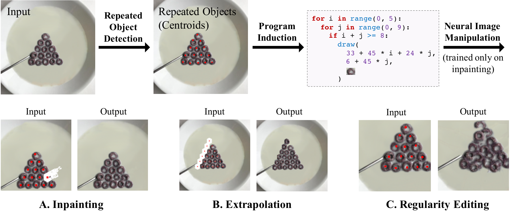
PG-IM combines repeated-object detection, symbolic programs describing spatial and attribute patterns, and an image-specific neural painter. A program supplies aligned source patches and determines where new objects belong. The same painter, trained for inpainting on the input image, can be used for extrapolation and regularity editing. Results favor the approach over the evaluated neural baselines on nearly regular patterns, but its language and repeated-pattern assumptions limit the range of images it can represent.
1 Introduction
Object identities and pairwise relations alone do not capture global repetition, boundaries, or alternating attributes. PG-IM represents these regularities with loops and conditions, then uses the representation to guide pixel synthesis. It evaluates inpainting, extrapolation, and regularity editing on rectified pattern and facade images, with additional qualitative Internet examples.
2 Related Work
The method combines ideas from image manipulation, procedural representations, and single-image learning.
Image manipulation.
Pixel and patch methods can fill local texture while missing object-level structure. Dataset-trained neural inpainting offers semantic priors but can introduce inappropriate content for an unusual repeated pattern. PG-IM instead supplies an explicit program for the particular image’s regularity.
Program induction and procedural modeling.
Program induction provides an interpretable description of loops, boundaries, and attributes. Unlike approaches focused on constrained synthetic imagery, this work applies such structure to selected natural patterns. The painter learns from the input image, although object detection still uses pretrained visual features.
Single-image learning.
A single image contains repeated statistics that can train an image-specific generator. The program adds global structure that a local texture prior may not preserve, such as a triangular arrangement rather than an unrestricted grid.

3 Program-Guided Image Manipulator
The pipeline detects repeated centroids, searches for a program that reconstructs their arrangement and attributes, then uses that program to condition a neural painter.
3.1 Repeated Object Detection
The detector starts from pretrained AlexNet features, identifies local activation peaks, votes for repeated displacements, and fits an implicit pattern model. This stage assumes approximately repeated lattice structure. The supplement restores the complete six-step procedure and its formulas.
3.2 Program Synthesizer
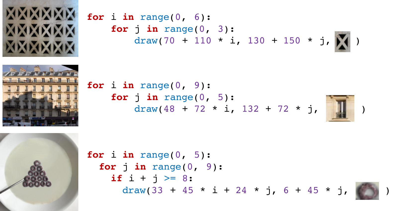
Detected centroids partition pixels into Voronoi cells. A program places objects at coordinates and assigns discrete appearance attributes. The search aims for a compact explanation of those detections rather than inferring an unrestricted scene model.
| Program | For1Stmt | |||||
|
|
| ||||
|
|
| ||||
| CondDrawStmt | If (Expr 0) { CondDrawStmt } | |||||
| CondDrawStmt | DrawStmt | |||||
|
|
| ||||
| AttributeExpr | Expr // Integer | |||||
| AttributeExpr | 1 If (Expr == 0) else 0 | |||||
| AttributeExpr | 1 If (Expr == 0 and Expr == 0) else 0 | |||||
| AttributeExpr | 1 If (Expr % Integer == 0) else 0 | |||||
| AttributeExpr | 1 If (Expr % Integer == 0 and Expr % Integer == 0) else 0 | |||||
| Expr | Integer * + Integer * + Integer |
Domain-specific language.
The domain-specific language contains nested loops, affine coordinate expressions, boundary conditions, drawing commands, and integer-valued attributes. The full grammar is retained in Table 1; patterns outside this grammar cannot be represented directly.
Program search.
Search is decomposed heuristically into lattice coordinates, boundary conditions, and appearance attributes. This reduces the combinatorial burden but is not a guarantee of a globally optimal program.
Lattice search.
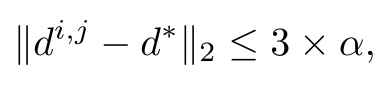
A five-parameter lattice maps loop indices to object coordinates. Its objective balances distances from detected centroids to reconstructed points against a penalty for excessive points. The regularization coefficient is five. The retained equation specifies the complete cost.
Equation 1
| (1) |
Condition search.
A minimum-cost assignment matches reconstructed and detected centroids. The convex hull of matched loop-index coordinates determines loop bounds and optional conditions. This handles rectangular and triangular boundaries while imposing a convexity assumption.
Attribute search.
Attribute expressions assign discrete labels as functions of loop indices. Search favors similar patches sharing a label and penalizes unnecessary distinct labels, with regularization strength ten. Integer and binary expression templates can represent alternating or grouped appearances; continuous attributes are not modeled.
Equation 2
| (2) |
3.3 Neural Painting Networks
The neural painting network treats manipulation as filling missing pixels. Program-derived object locations make it possible to reuse an inpainting-trained model for the other tasks.
Patch aggregation.
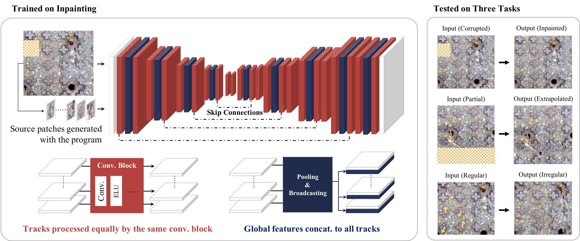
To fill one object, the system translates other objects to align their centroids with the missing region. These aligned source images and the corrupted input form a variable-size stack from which the painter can recover suitable content.
Architecture.
A shared-weight U-Net processes every source track. Intermediate max pooling forms a global feature that is broadcast back to all tracks, making the architecture insensitive to track order and able to handle different numbers of source images. Skip connections preserve local detail. The complete layer listing is retained in the supplement.
Extrapolation and regularity editing as recurrent inpainting.
Extrapolation edits program bounds to identify new objects, then fills them one at a time, using earlier predictions as context. Regularity editing moves each Voronoi cell with its centroid and fills the resulting gaps. This reuses the trained painter but does not imply arbitrary structural edits are supported.
Training.
Each input image receives its own trained painter, using reconstruction and adversarial losses. Training samples corrupted patches from that image rather than learning the painter once for all test images. The pretrained feature detector remains an external learned component.
4 Experiments and Applications
Quantitative inpainting and qualitative extrapolation and regularity editing compare PG-IM with patch-based and neural baselines. The supplemental ablations test source patches, recurrent filling, and attributes.
4.1 Dataset
The experiments use 48 rectified Nearly-Regular Pattern images and 109 rectified facade images. These are selected structured domains, not a representative sample of unrestricted natural scenes.
4.2 Baselines
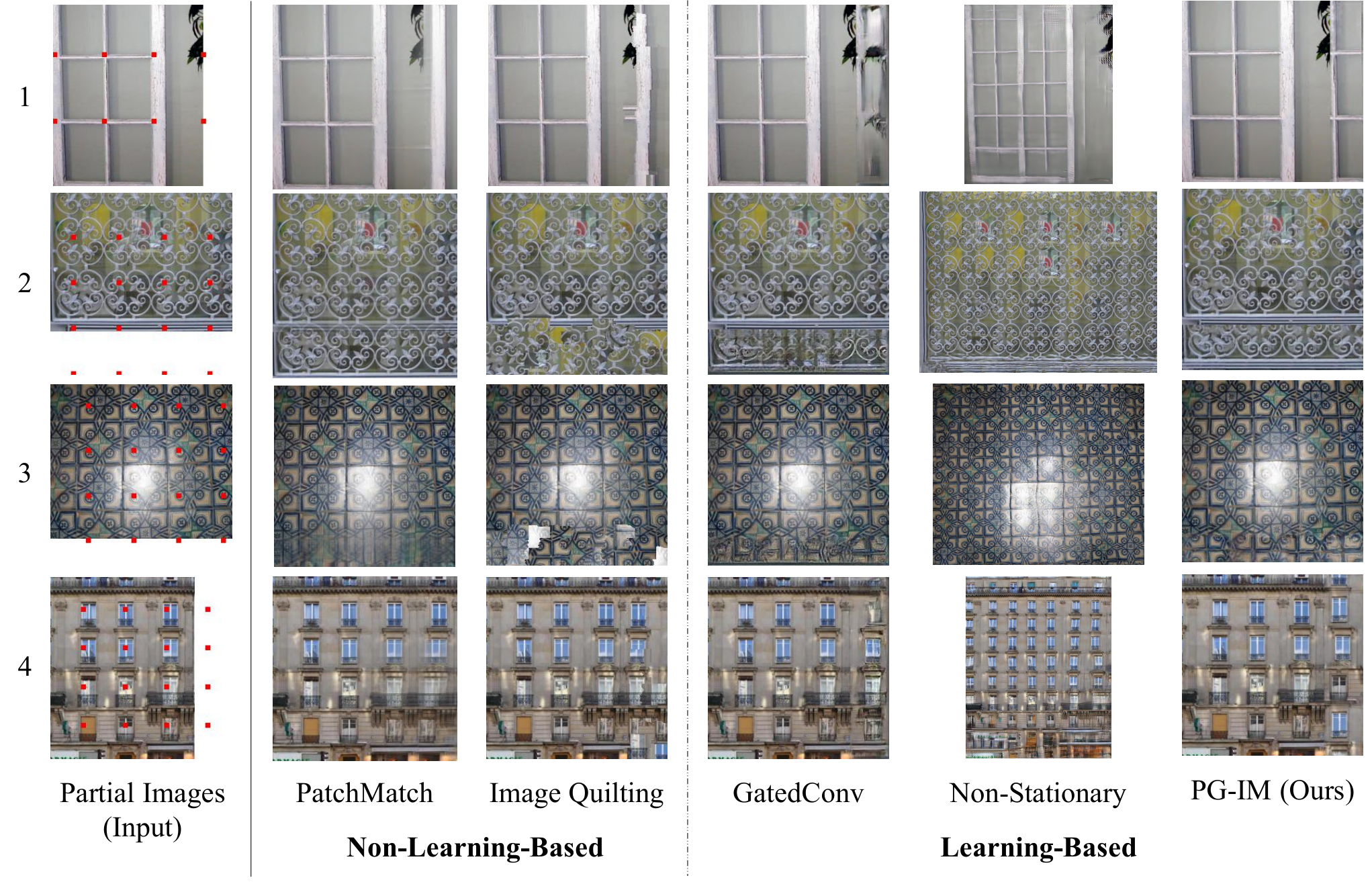
Baselines include Image Quilting, PatchMatch, pretrained GatedConv, and image-specific Non-Stationary texture synthesis. Hyperparameters are selected across test images, while image-specific networks are trained separately. Some baselines need user-specified extrapolation masks, whereas PG-IM derives positions from its program; this is a difference in task interface as well as synthesis.
| Method | L1 Mean (Std.) | Inception Score |
|---|---|---|
| Nearly-Regular Patterns [22] | ||
| Image Quilting [11] | 12.30 (2.903) | 1.253 |
| PatchMatch [6] | 83.91 (17.62) | 1.210 |
| GatedConv [48] | 50.45 (16.46) | 1.196 |
| Non-Stationary [50] | 103.7 (23.87) | 1.186 |
| PG-IM (ours) | 21.48 (5.375) | 1.229 |
| Facade [39] | ||
| Image Quilting [11] | 13.50 (6.379) | 1.217 |
| PatchMatch [6] | 81.35 (25.28) | 1.219 |
| GatedConv [48] | 26.26 (133.9) | 1.186 |
| Non-Stationary [50] | 133.9 (39.75) | 1.199 |
| PG-IM (ours) | 14.40 (7.781) | 1.218 |
4.3 Inpainting
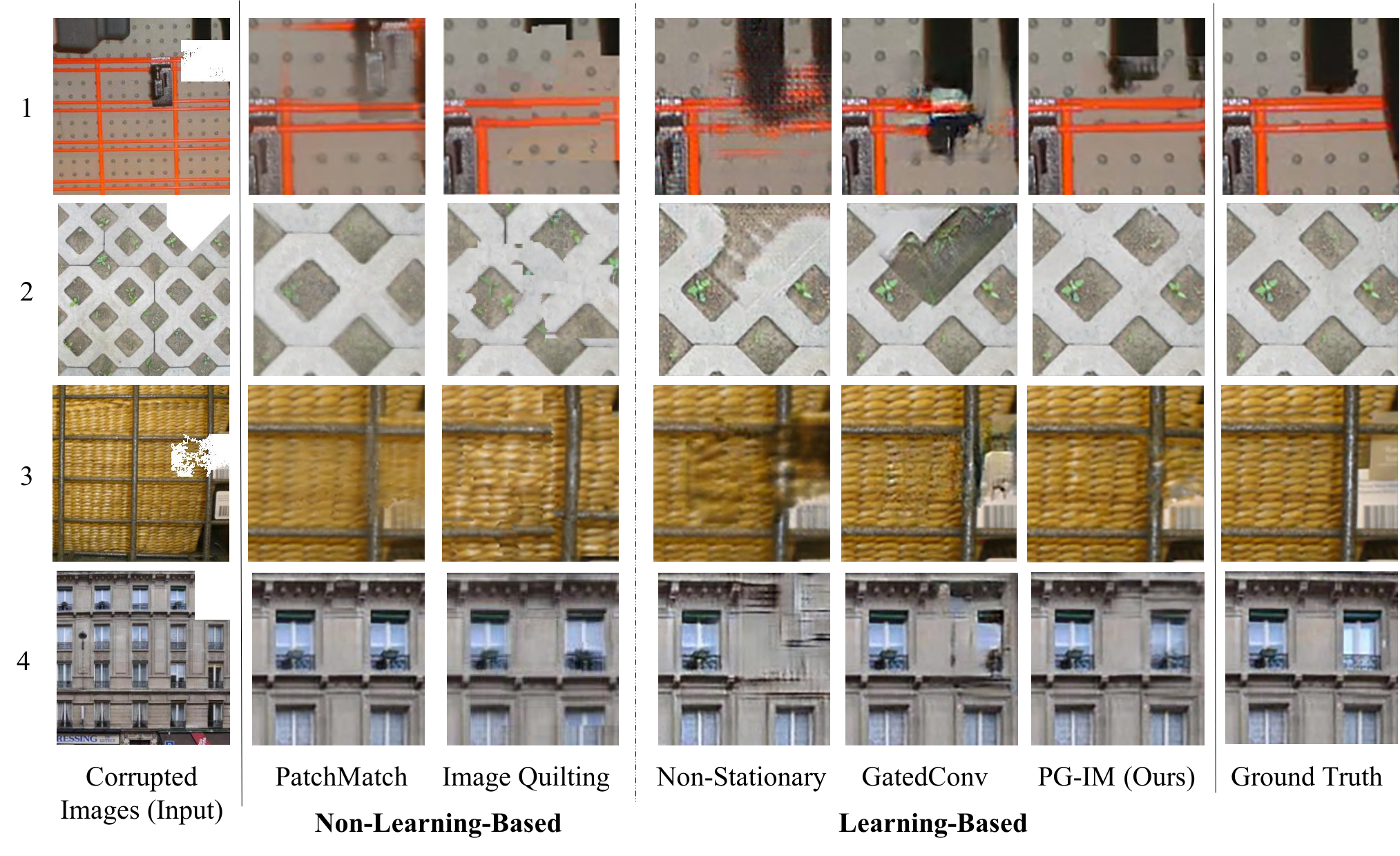
Each image is corrupted 100 times, with test patches withheld from training. PG-IM improves reconstruction and Inception scores over the reported neural baselines, but Image Quilting has lower L1 error on both datasets. Qualitative examples motivate the value of structural consistency despite that metric difference. The roughly 100 ms neural inference time excludes per-image training; it should not be read as the complete cost of processing a new image. The source’s table contains an unusually large GatedConv standard deviation, which is retained rather than corrected without evidence.
4.4 Extrapolation
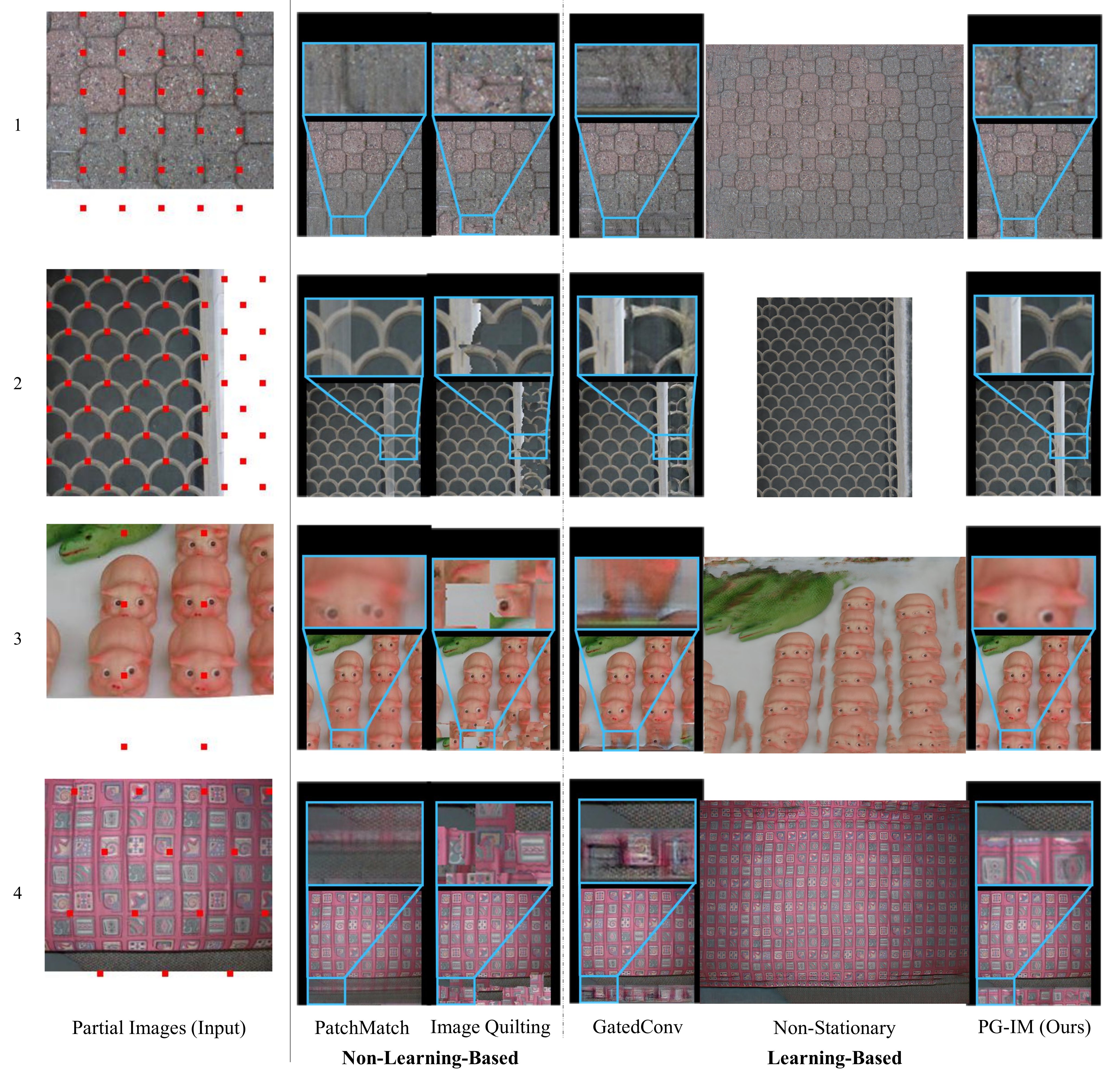
Extending loop ranges or relaxing conditions supplies new object locations. The visual comparisons show examples where PG-IM preserves layout and boundary continuity while baselines blur or introduce inconsistent content. These selected examples support the proposed mechanism but do not provide a quantitative generalization rate.
4.5 Image Regularity Editing
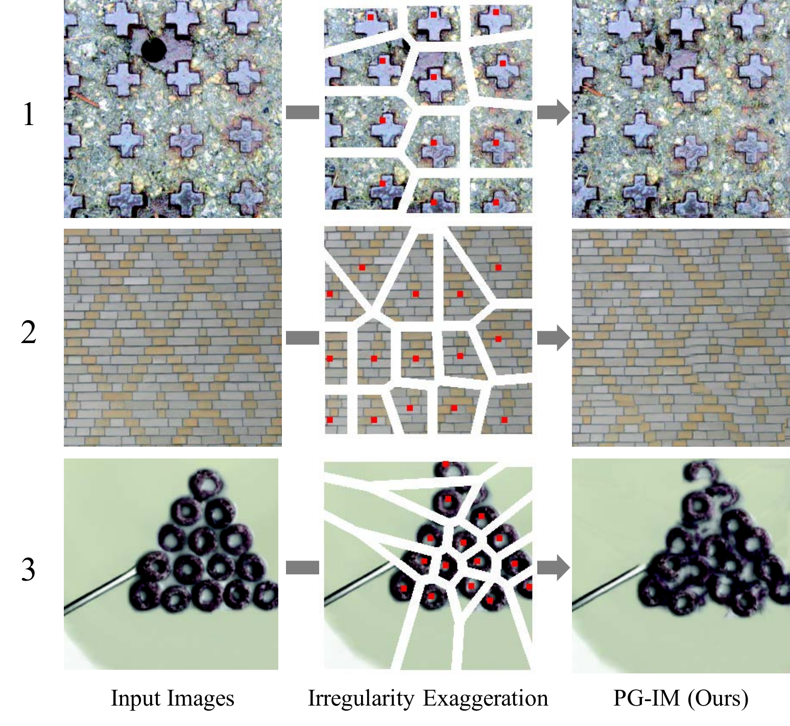
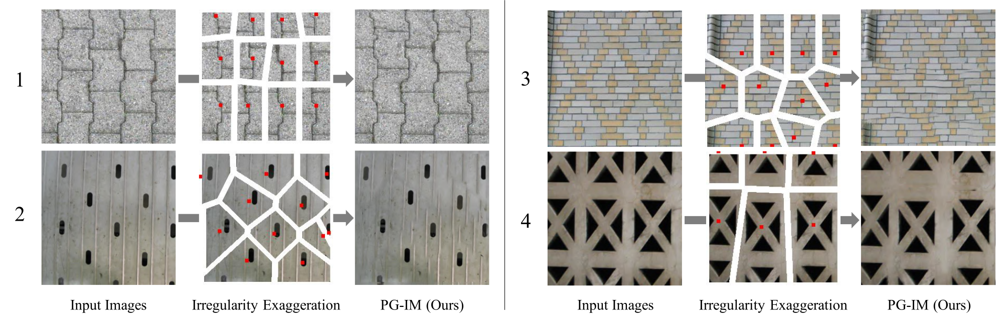
Irregularity editing magnifies the difference between detected centroids and ideal program positions. The corresponding image cells move with the objects, and recurrent inpainting repairs gaps. The edits are constrained by the inferred pattern.
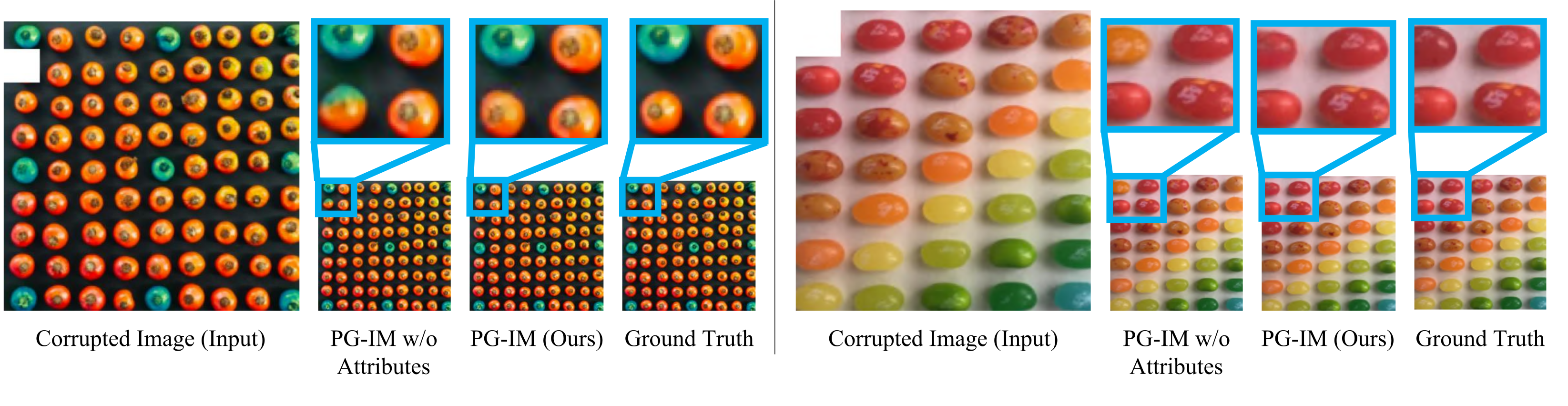
4.6 Attribute Regularity
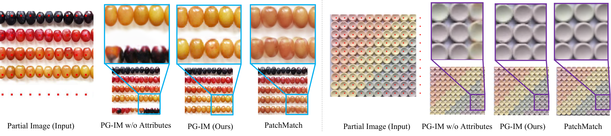
Attribute-aware source selection avoids mixing patches that occupy different roles in a global color pattern. The illustrated ablations show color inconsistencies without this selection. Attributes are discrete, leaving continuous appearance variation outside the current representation.
5 Discussion
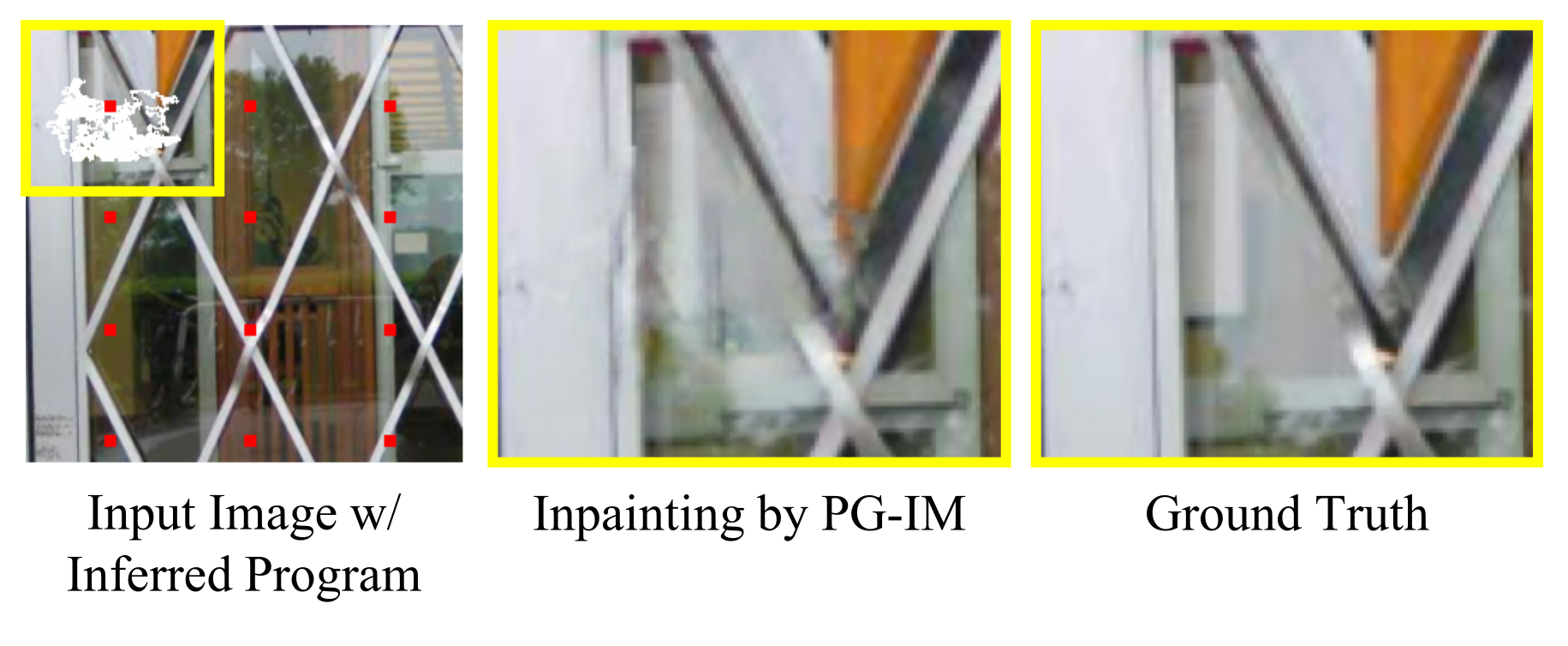
PG-IM combines explicit regularity with local image synthesis, but its representational language restricts supported patterns. Rotation patterns and richer continuous attributes are left for future work. It also cannot infer semantically new structures, such as adding a roof to repeated windows, from repetition alone. The supplement provides a failure caused by reflection and transmission.
Supplement A. Implementation details
The supplement specifies the detector, adaptive discriminator, recurrent generation, and per-image training procedure.
A.1 Repeated object detection
The detector finds feature-map peaks, votes for repeated displacements, filters inconsistent vectors, weights feature maps, optimizes lattice offset, and lets activations vote for individual centroids. The six original displayed formulas are retained below with editorial labels S1-S6; these labels are added for navigation. The final local vote allows departures from a perfectly regular lattice.
Equations S1–S6





A.2 Adaptive discriminator depth
AdaPatchGAN adapts discriminator depth to the inferred object-patch scale, adding layers until its receptive field covers a typical patch. This avoids using one fixed receptive field for both small repeated textures and large objects.
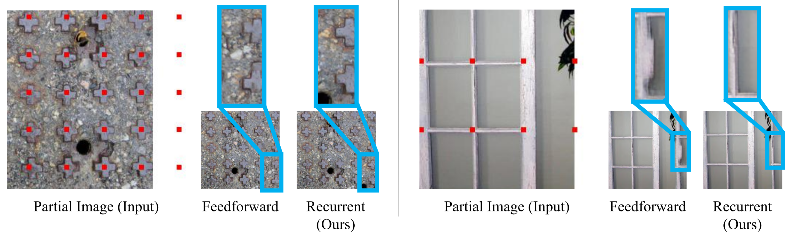
A.3 Recurrent extrapolation
Filling an entire extrapolation strip at once differs from the localized corruption used for training. Recurrent filling instead generates one object at a time and includes completed objects in later context. The ablation below illustrates the resulting reduction in distorted objects.
A.4 Training parameters
Training follows the pix2pix setup but does not decay the learning rate after 100 epochs. Each epoch contains 1,000 randomly cropped samples from the same image, and the authors report convergence within roughly 150 epochs. This substantial image-specific training cost is separate from the final forward-pass timing.
Supplement B. Ablations
The three ablations isolate the role of program-derived source patches, recurrent inference, and discrete attributes. They are visual comparisons rather than a broad statistical decomposition of performance.
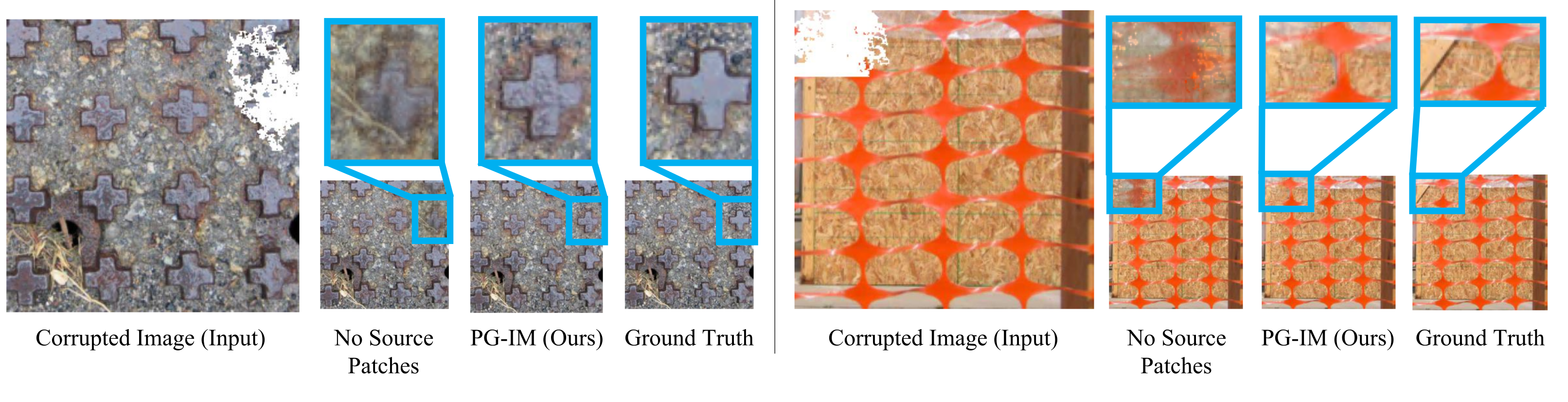
B.1 Source patches
Without aligned source patches, the painter can restore background while omitting the object. The two examples show the program’s value in supplying an intact counterpart of a completely corrupted repeated element.
B.2 Recurrent inpainting
Recurrent extrapolation better matches the local inpainting task used in training. Filling the whole stripe in one pass produces distorted objects in the illustrated comparisons.
B.3 Object attributes
The attribute ablation mixes nearby colors even when the global arrangement requires one particular color. Restricting source patches to the appropriate attribute preserves the repeated pattern in the tomato and candy examples.
Supplement C. Additional experiments
The additional galleries retain every published comparison, including the failure case and the fine-tuned baseline.
C.1 Additional inpainting results
Six additional inpainting examples compare the method with all listed baselines and ground truth. The examples emphasize preserving whole repeated structures rather than only plausible local texture.
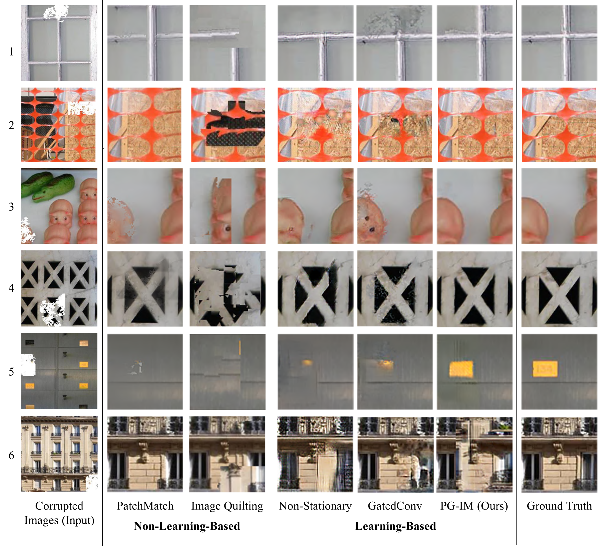
C.2 Additional extrapolation results
Four additional extrapolation examples compare boundary continuity and pattern extension. The baselines differ in whether they modify existing content or merely fill the newly exposed region, which matters when interpreting visual differences.
C.3 Regularity editing
The source doubles irregularity displacement vectors and randomly flips their signs, then shifts patches and fills gaps. All four examples remain available for inspecting the effect.
C.4 Failure cases
Transmission and reflections make corresponding objects visually inconsistent. In this example, the model generates non-photorealistic content despite a plausible repeated layout, exposing the limits of copying internal statistics.
C.5 Fine-tuned baseline
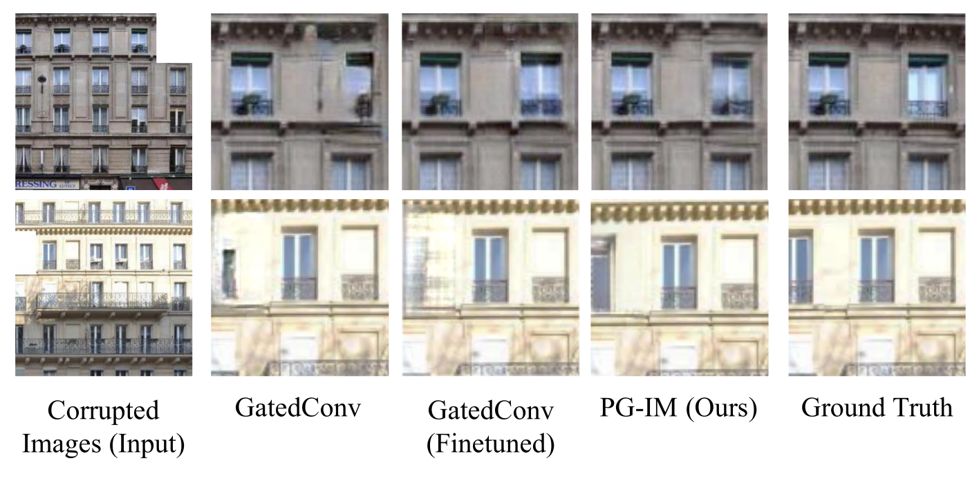
Fine-tuning GatedConv on 50 facade images improves its Inception score from 1.187 to 1.191, versus 1.210 for the image-specific PG-IM comparison. Structured windows can remain problematic after fine-tuning. The training regimes differ, so this is not an equal-data comparison.
Appendix: Complete generator architecture
The complete commented generator listing preserves channel counts, kernel sizes, strides, padding, pooling across tracks, and skip connections. It spans the final two PDF pages and is retained as selectable code.
('1', ReppadConv2d(3, 64, 3, stride=1, padding=1)),
           ('1a', nn.ELU()),
           # 2: maxpool across tracks
           # 3: concat 2
           ('4:+pool', ReppadConv2d(128, 96, 1, stride=1)),
           ('4a', nn.ELU()),
           ('5', ReppadConv2d(96, 96, 4, stride=2, padding=1)),
           ('5a', nn.ELU()),
           # 6: maxpool across tracks
           # 7: concat 6
           ('8:+pool', ReppadConv2d(192, 128, 1, stride=1)),
           ('8a', nn.ELU()),
           ('9', ReppadConv2d(128, 128, 4, stride=2, padding=1)),
           ('9a', nn.ELU()),
           # 10: maxpool across tracks
           # 11: concat 10
           ('12:+pool', ReppadConv2d(256, 256, 1, stride=1)),
           ('12a', nn.ELU()),
           ('13', ReppadConv2d(256, 256, 4, stride=2, padding=1)),
           ('13a', nn.ELU()),
           # 14: maxpool across tracks
           # 15: concat 14
           ('16:+pool', ReppadConv2d(512, 384, 1, stride=1)),
           ('16a', nn.ELU()),
           ('17', ReppadConv2d(384, 384, 4, stride=2, padding=1)),
           ('17a', nn.ELU()),
           ('18', ReppadConv2d(384, 384, 3, stride=1, padding=1)),
           ('18a', nn.ELU()),
           # ----------------
           ('19', nn.ConvTranspose2d(384, 384, 4, stride=2, padding=1)),
           ('19a', nn.ELU()),
           # 20: maxpool across tracks
           # 21: concat 16a, 20
           ('22:+pool+16a', ReppadConv2d(1152, 384, 1, stride=1)),
           ('22a', nn.ELU()),
           ('23', ReppadConv2d(384, 384, 3, stride=1, padding=1)),
           ('23a', nn.ELU()),
           ('24', nn.ConvTranspose2d(384, 256, 4, stride=2, padding=1)),
           ('24a', nn.ELU()),
           # 25: maxpool across tracks
           # 26: concat 12a, 25
           ('27:+pool+12a', ReppadConv2d(768, 256, 1, stride=1)),
           ('27a', nn.ELU()),
           ('28', ReppadConv2d(256, 256, 3, stride=1, padding=1)),
           ('28a', nn.ELU()),
           ('29', nn.ConvTranspose2d(256, 192, 4, stride=2, padding=1)),
           ('29a', nn.ELU()),
           # 30: maxpool across tracks
           # 31: concat 8a, 30
           ('32:+pool+8a', ReppadConv2d(512, 192, 1, stride=1)),
           ('32a', nn.ELU()),
           ('33', ReppadConv2d(192, 192, 3, stride=1, padding=1)),
           ('33a', nn.ELU()),
           ('34', nn.ConvTranspose2d(192, 96, 4, stride=2, padding=1)),
           ('34a', nn.ELU()),
           # 35: maxpool across tracks
# 36: concat 1a, 35
('37:+pool+1a', ReppadConv2d(256, 96, 1, stride=1)),
('37a', nn.ELU()),
('38', ReppadConv2d(96, 96, 3, stride=1, padding=1)),
('38a', nn.ELU()),
# 39: maxpool across tracks
('40:pool', ReppadConv2d(96, 64, 3, stride=1, padding=1)),
('40a', nn.ELU()),
('41', ReppadConv2d(64, nch_out, 3, stride=1, padding=1)),