Overview
The paper and complete supplement are included. The supplement compares baseline supervision, details implementation and model selection, checks parser-derived evaluation targets, and retains all eleven example parse trees.
At a glance
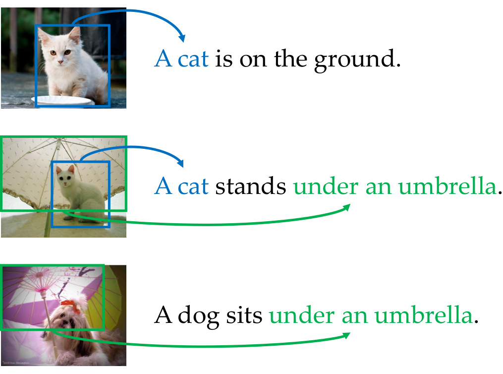
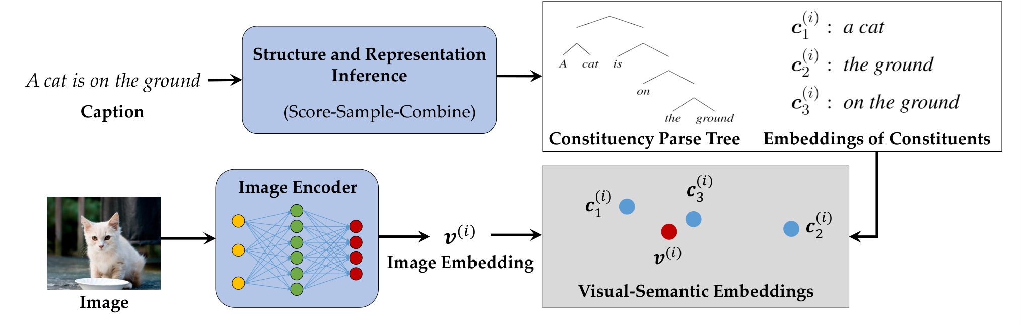
VG-NSL learns binary constituency trees from images paired with captions, without training on labeled trees or part-of-speech tags. It rewards constituents whose embeddings match the associated image, coupling syntax induction with visually grounded representation learning. A language-specific head-initial bias improves results. In caption-domain experiments, the method is more stable across random seeds and more data-efficient than selected text-only baselines. These are grounded-caption results, not evidence of general syntax acquisition from arbitrary language.
1 Introduction
A visually meaningful phrase can provide a cue that its words form a constituent. VG-NSL repeatedly combines adjacent spans, represents the resulting constituents, and matches them to images. Training uses visual concreteness to guide these decisions; parsing at test time needs only text. The work evaluates tree agreement, seed stability, phrase types, data efficiency, and learned concreteness in English, with additional German and French caption experiments.
2 Related Work
Linguistic structure induction from text.
Earlier latent-tree models learn from downstream tasks or language modeling. Many are unstable across random seeds or recover structures that differ from conventional syntax. Other unsupervised grammar methods rely on gold part-of-speech tags. VG-NSL replaces explicit syntactic annotations with paired visual evidence, while retaining pretrained visual features and structural inductive biases.
Grounded language acquisition.
Grounded language learning has used image, video, and reasoning tasks, often with labeled visual categories or hand-designed rules. This method borrows image-text alignment objectives but uses their signal to induce constituency structure.
Concreteness estimation.
Concreteness measures how readily a word or phrase corresponds to perceptible things, properties, or events. Unlike prior word-level estimates, VG-NSL scores composed spans and uses these scores during parsing.
3 Visually Grounded Neural Syntax Learner
A textual module constructs trees and recursively represents their constituents. A visual-semantic module aligns those representations with paired images. The two modules alternate optimization, so better grounding can guide structure and better structure can improve alignment.
3.1 Textual Representations and Structures
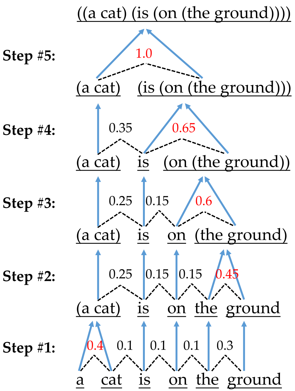
For a sentence of n tokens, the parser makes n−1 adjacent-span merges. A two-layer network scores every possible merge; training samples from the scores, while test-time inference chooses the maximum. Each merged representation is the normalized sum of its children. This deliberately simple composition discourages the encoder from ignoring all but a salient word. A complete binary tree contains 2n−1 constituents when individual words are included.
Equations
| score | |||
3.2 Visual-Semantic Embeddings
A learned projection maps image features into the same space as text constituents. Cosine similarity measures their match. The alignment stage treats a tree as a set of constituents rather than directly modeling its topology.
Equation
3.3 Training
A triplet-ranking loss trains image and constituent representations to distinguish matched pairs from mismatches. REINFORCE updates the discrete merge policy. Its reward measures how concretely a newly formed span matches the paired image relative to alternatives. Images supervise training but are not needed when the learned parser is applied to new text. The complete matching, concreteness, and reward formulas are retained.
Equations 1–2
| (1) |
| (2) |
3.4 The Head-Initial Inductive Bias
The head-initial variant penalizes merging an abstract right constituent with material to its left, encouraging heads such as prepositions to combine with following complements. This is an explicit language-specific bias, not structure learned entirely from data. The paper cautions that the same bias does not transfer directly to head-final languages such as Japanese.
Equations 3
| (3) | ||||
4 Experiments
Evaluation separates agreement with reference trees from self-agreement across independent training runs. It also examines individual phrase types, training-data requirements, concreteness estimates, and language transfer.
4.1 Data Sets and Metrics
MSCOCO contains 82,783 training images and 1,000 images each for development and test, with five captions per image. Test reference trees are generated by the supervised Benepar parser. A separate manual check on 50 captions finds 95.65 F1 agreement with Benepar. Reported constituency F1 aggregates spans across the dataset rather than averaging sentence-level F1. The evaluation stays within caption language; newspaper-domain parsing is left for future work.
4.2 Baselines
Baselines vary in objective and available information. The tables explicitly distinguish extra linguistic labels or corpora from paired-image supervision and pretrained visual features.
| Model | NP | VP | PP | ADJP | Avg. | Self | |||||
| Random | 47.3 | ±0.3 | 10.5 | ±0.4 | 17.3 | ±0.7 | 33.5 | ±0.8 | 27.1 | ±0.2 | 32.4 |
| Left | 51.4 | 1.8 | 0.2 | 16.0 | N/A | ||||||
| Right | 32.2 | 23.4 | 18.7 | 14.4 | N/A | ||||||
| PMI | 54.2 | 16.0 | 14.3 | 39.2 | N/A | ||||||
| PRPN (Shen et al., 2018a) | 72.8 | ±9.7 | 33.0 | ±9.1 | 61.6 | ±9.9 | 35.4 | ±4.3 | 52.5 | ±2.6 | 60.3 |
| ON-LSTM (Shen et al., 2019) | 74.4 | ±7.1 | 11.8 | ±5.6 | 41.3 | ±16.4 | 44.0 | ±14.0 | 45.5 | ±3.3 | 69.3 |
| Gumbel (Choi et al., 2018)† | 50.4 | ±0.3 | 8.7 | ±0.3 | 15.5 | ±0.0 | 34.8 | ±1.6 | 27.9 | ±0.2 | 40.1 |
| VG-NSL (ours)† | 79.6 | ±0.4 | 26.2 | ±0.4 | 42.0 | ±0.6 | 22.0 | ±0.4 | 50.4 | ±0.3 | 87.1 |
| VG-NSL+HI (ours)† | 74.6 | ±0.5 | 32.5 | ±1.5 | 66.5 | ±1.2 | 21.7 | ±1.1 | 53.3 | ±0.2 | 90.2 |
| VG-NSL+HI+FastText (ours)*† | 78.8 | ±0.5 | 24.4 | ±0.9 | 65.6 | ±1.1 | 22.0 | ±0.7 | 54.4 | ±0.4 | 89.8 |
| Concreteness estimation–based models | |||||||||||
| Turney et al. (2011)* | 65.5 | 30.8 | 35.3 | 30.4 | 42.5 | N/A | |||||
| Turney et al. (2011)+HI* | 74.5 | 26.2 | 47.6 | 25.6 | 48.9 | N/A | |||||
| Brysbaert et al. (2014)* | 54.1 | 27.8 | 27.0 | 33.1 | 34.1 | N/A | |||||
| Brysbaert et al. (2014)+HI* | 73.4 | 23.9 | 50.0 | 26.1 | 47.9 | N/A | |||||
| Hessel et al. (2018)† | 50.9 | 21.7 | 32.8 | 27.5 | 33.2 | N/A | |||||
| Hessel et al. (2018)+HI† | 72.5 | 34.4 | 65.8 | 26.2 | 52.9 | N/A | |||||
Trivial tree structures.
Random binary, purely left-branching, and purely right-branching trees provide structural baselines without linguistic training.
Syntax acquisition by language modeling and statistics.
PRPN and ON-LSTM induce syntactic distances while optimizing language modeling. A separate statistical baseline uses negative pointwise mutual information between neighboring words as a distance. Each distance sequence is converted recursively into a binary tree.
Syntax acquisition from downstream tasks.
A Gumbel-softmax latent-tree caption encoder is trained for image-caption retrieval, testing whether a downstream alignment objective alone produces useful structure.
Syntax acquisition from concreteness estimation.
Additional baselines merge spans using externally estimated word concreteness. They include semi-supervised, crowdsourced, and multimodal estimates, with and without a head-initial bias. Their supervision differs, so they should not all be described as equally annotation-free.
4.3 Implementation Details
Word and constituent embeddings have 512 dimensions. A pretrained ResNet-101 supplies 2,048-dimensional image vectors, projected into the common space. The merge scorer has a 128-dimensional hidden layer. VG-NSL trains for 30 epochs with Adam, reducing the learning rate from 0.0005 to 0.00005 after 15 epochs. Hyperparameters are tuned through agreement among five random-seed runs.
4.4 Results: Unsupervised Constituency Parsing
VG-NSL with the head-initial bias performs best among the compared models without extra syntactic labels, particularly on noun and prepositional phrases. PRPN remains a competitive text-only baseline but is less stable. ON-LSTM performs poorly overall on these captions despite its strong newspaper-domain results, while remaining strong on adjective phrases. Adding pretrained FastText vectors raises mean F1 to 54.4%; that variant introduces additional text pretraining.
4.5 Results: Data Efficiency
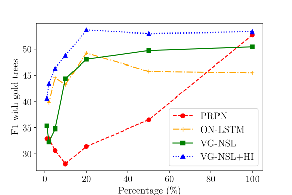
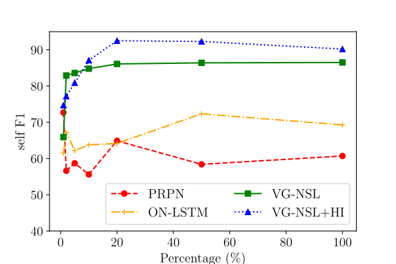
Training fractions range from 1% to 100%. VG-NSL matches the fully trained PRPN baseline using about 20% of the caption data and becomes more consistent across seeds as data increases. The prose also describes this setting as 8K images with 40K captions, which does not equal 20% of the stated 82,783-image training set; Figure 4 preserves the source’s percentage-axis results without resolving that inconsistency.
4.6 Analysis: Consistency with Linguistic Concreteness
Word concreteness is averaged over associated images and compared with existing estimates or human judgments. Correlations are computed on the 100 most frequent test words, averaged over five runs. Agreement is substantial in this selected vocabulary, but does not establish equivalent concreteness judgments for rare words or abstract language.
| Model/method | VG-NSL | (+HI) |
| Turney et al. (2011) | 0.74 | 0.72 |
| Brysbaert et al. (2014) | 0.71 | 0.71 |
| Hessel et al. (2018) | 0.84 | 0.85 |
4.7 Analysis: Self-Agreement F 1 Score as the Criterion for Model Selection
Model selection maximizes pairwise tree agreement across five independently initialized runs and nearby checkpoints. It yields 50.4 mean F1 for VG-NSL versus 47.7 with image-retrieval-based selection; the head-initial variant changes from 53.1 to 53.3. Self-agreement measures consistency, which alone need not imply correctness. PRPN and ON-LSTM were not tuned with this criterion because repeated evaluation was expensive, so the comparison does not isolate architecture from all selection differences.
| Model | Criterion | Avg. | Self |
| VG-NSL | Self | 50.4 ±0.3 | 87.1 |
| VG-NSL | R@1 | 47.7 ±0.6 | 83.4 |
| VG-NSL+HI | Self | 53.3 ±0.2 | 90.2 |
| VG-NSL+HI | R@1 | 53.1 ±0.2 | 88.7 |
Equations
4.8 Extension to Multiple Languages
Multi 30K provides 29,000 training images,1,014 development images, and 1,000 test images, with one caption per language per image. The head-initial variant performs best among the reported models in English, German, and French. These scores are not directly comparable with MSCOCO because the amount and distribution of caption data differ.
| Model | EN | DE | FR | |||
| PRPN | 30.8 | ±17.9 | 31.5 | ±8.9 | 27.5 | ±7.0 |
| ON-LSTM | 38.7 | ±12.7 | 34.9 | ±12.3 | 27.7 | ±5.6 |
| VG-NSL | 33.5 | ±0.2 | 36.3 | ±0.2 | 34.3 | ±0.6 |
| VG-NSL+HI | 38.7 | ±0.2 | 38.3 | ±0.2 | 38.1 | ±0.6 |
5 Discussion
Visual grounding can make caption-domain latent-tree learning more accurate and reproducible in these experiments. Remaining limitations include static-scene supervision, whole-image alignment, shared syntax/semantics representations, reliance on a head-direction bias, and evaluation against mostly parser-generated targets. Structured visual representations, other modalities, and integration with text-only learning are proposed extensions.
Acknowledgement
The authors acknowledge Allyson Ettinger and the reviewers.
Appendix A Overview of Models for Constituency Parsing without Explicit Syntactic Supervision
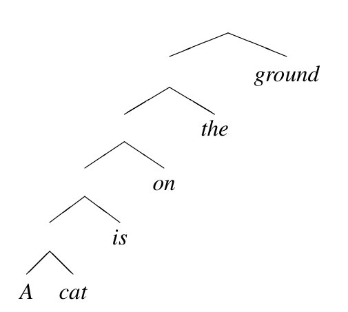
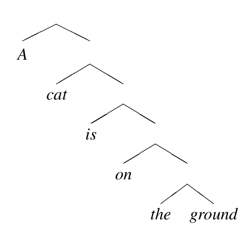
Table 5 retains the complete comparison of objectives, extra labels, additional corpora, multimodal inputs, and stochastic behavior. All listed multimodal methods use pretrained visual feature extractors. Figure 5 retains the contrasting left- and right-branching examples.
| Model | Objective | Extra Label | Multi- | Stochastic | Extra | ||
| modal | Corpus | ||||||
| CCM Klein and Manning (2002)* | MAP | POS | ✗ | ✓ | ✗ | ||
| DMV-CCM Klein and Manning (2005)* | MAP | POS | ✗ | ✓ | ✗ | ||
| U-DOP Bod (2006b)* | Probability Estimation | POS | ✗ | ✗ | ✗ | ||
| UML-DOP Bod (2006a)* | MAP | POS | ✗ | ✓ | ✗ | ||
| PMI | N/A | ✗ | ✗ | ✗ | ✗ | ||
| Random | N/A | ✗ | ✗ | ✓ | ✗ | ||
| Left | N/A | ✗ | ✗ | ✗ | ✗ | ||
| Right | N/A | ✗ | ✗ | ✗ | ✗ | ||
| PRPN Shen et al. (2018a) | LM | ✗ | ✗ | ✓ | ✗ | ||
| ON-LSTM Shen et al. (2019) | LM | ✗ | ✗ | ✓ | ✗ | ||
| Gumbel softmaxChoi et al. (2018) | Cross-modal Retrieval | ✗ | ✓ | ✓ | ✗ | ||
| VG-NSL (ours) | Cross-modal Retrieval | ✗ | ✓ | ✓ | ✗ | ||
| VG-NSL+HI (ours) | Cross-modal Retrieval | ✗ | ✓ | ✓ | ✗ | ||
| Concreteness estimation based models | |||||||
| Turney et al. (2011)* | N/A |
|
✗ | ✗ | ✓ | ||
| Turney et al. (2011)+HI* | N/A |
|
✗ | ✗ | ✓ | ||
| Brysbaert et al. (2014)* | N/A |
|
✗ | ✗ | ✗ | ||
| Brysbaert et al. (2014)+HI* | N/A |
|
✗ | ✗ | ✗ | ||
| Hessel et al. (2018) | N/A | ✗ | ✓ | ✗ | ✗ | ||
| Hessel et al. (2018)+HI | N/A | ✗ | ✓ | ✗ | ✗ | ||
Appendix B Implementation Details for VG-NSL
The visual-semantic module follows the VSE++ implementation, with margin 0.2 and a shared vocabulary of 10,000 frequent MSCOCO words. Out-of-vocabulary words receive the same unseen-word treatment across applicable methods.
Hyperparameter tuning.
Hyperparameters are selected by self-agreement rather than labeled parsing accuracy. The head-initial penalty is searched over 1,2,5,10,20,50, and 100; the selected value is 20.
Appendix C Implementation Details for Baselines
Trivial tree structures.
Random trees repeatedly merge randomly chosen neighboring constituents; fixed left- and right-branching trees supply deterministic alternatives. The original examples remain in Figure 5.
Parsing-Reading-Predict Network (PRPN).
PRPN uses 512-dimensional hidden layers, Adam, and a search over one to three layers and three learning rates. Training budgets are 100 epochs on MSCOCO and 1,000 on Multi 30K, with language-model perplexity used for tuning and stopping.
Ordered Neurons (ON-LSTM).
ON-LSTM uses three 512-dimensional layers and chunk size 16; trees come from the second layer’s gates. Both Adam and stochastic gradient descent are explored with multiple learning rates. Training budgets and selection use language-model perplexity as for PRPN.
PMI based constituency parsing.
The statistical baseline estimates adjacent-word mutual information from training captions, negates it into a syntactic distance, and recursively splits at the largest distance. Algorithm 1 retains every step.
Gumbel-softmax based latent tree.
The Gumbel-softmax baseline inserts a latent-tree text encoder into the visual-semantic retrieval system. Tables and figures retain its comparison with the proposed policy and concreteness baselines.
| Turney et al. (2011) | Brysbaert et al. (2014) | Hessel et al. (2018) | VG-NSL+HI | |
| Turney et al. (2011) | 1.00 | 0.84 | 0.58 | 0.72 |
| Brysbaert et al. (2014) | 0.84 | 1.00 | 0.55 | 0.71 |
| Hessel et al. (2018) | 0.58 | 0.55 | 1.00 | 0.85 |
| VG-NSL+HI | 0.72 | 0.71 | 0.85 | 1.00 |
Concreteness estimation.
The semi-supervised concreteness baseline uses 4,295 manually scored words and Wikipedia word associations. Crowdsourced scores are taken from the released human-rating dataset; the multimodal baseline is estimated on MSCOCO. These sources are explicitly distinguished from VG-NSL’s paired-caption training signal.
Constituency parsing with concreteness scores.
Word-concreteness scores are normalized to[−1,1], with unseen words assigned−1. Adjacent spans with the largest average score are merged, and their new score is the children’s mean. The head-initial variant weights the right constituent by 20 for selection while leaving the composed score unweighted. Algorithm 2 preserves the complete procedure.
Equation
Appendix D Details of Manual Ground Truth Evaluation
Fifty randomly selected test captions were manually parsed without looking at Benepar outputs or images. These annotations cover tree structure rather than constituent categories. Benepar agrees at 95.65 F1; remaining examples often involve commonsense-dependent attachment ambiguities. This supports its use as a reference on a small sample, while retaining the limits of that validation.
Appendix E Concreteness by Different Models
E.1 Correlation between Different Concreteness Estimations
The full correlation matrix compares the linguistic, human-rated, multimodal, and VG-NSL concreteness measures on the same 100 frequent test words. VG-NSL correlates more strongly with the linguistic and human-rated measures than the compared multimodal baseline does.
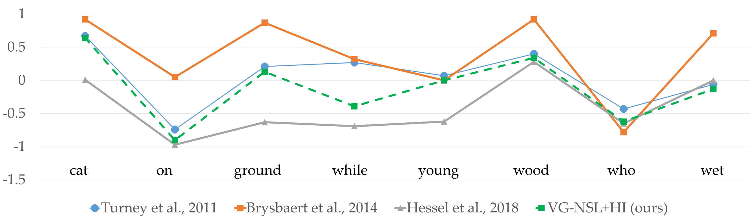
E.2 Concreteness Scores of Sample Words by Different Methods
Figure 6 preserves all normalized scores for the selected example words, illustrating both broad agreement and differences between methods.
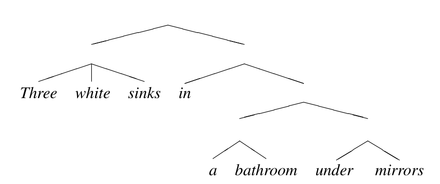
Appendix F Sample Trees Generated by VG-NSL
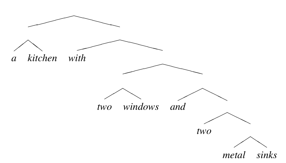
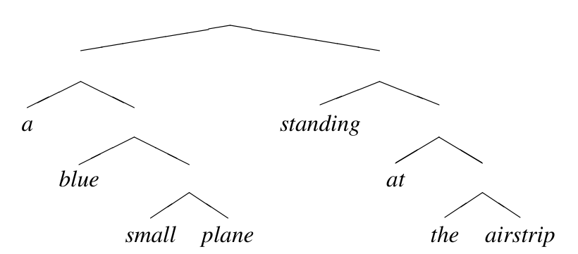
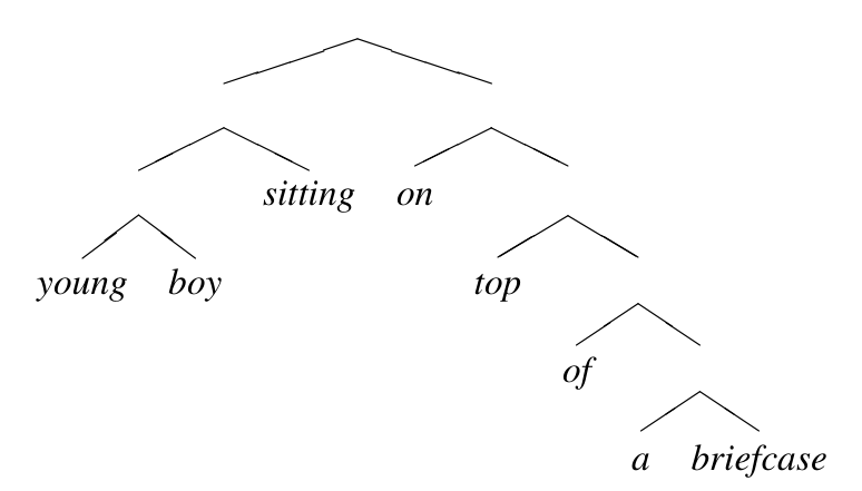
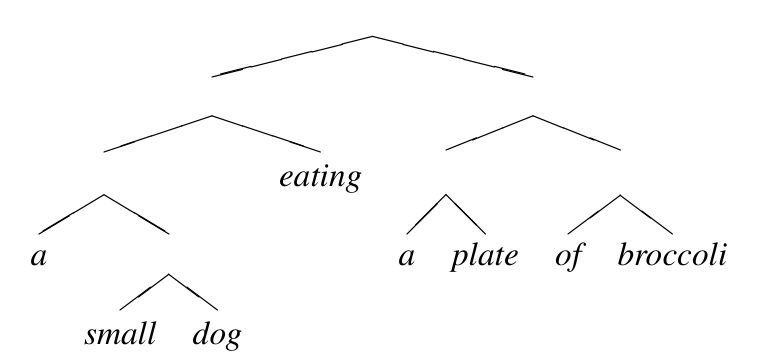
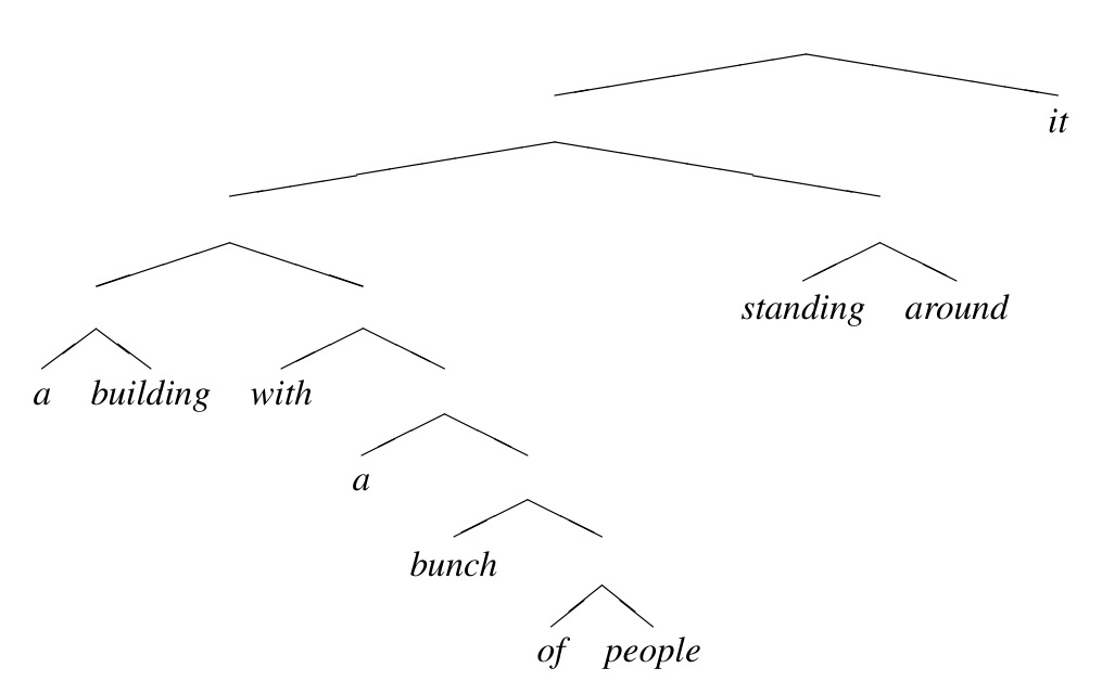
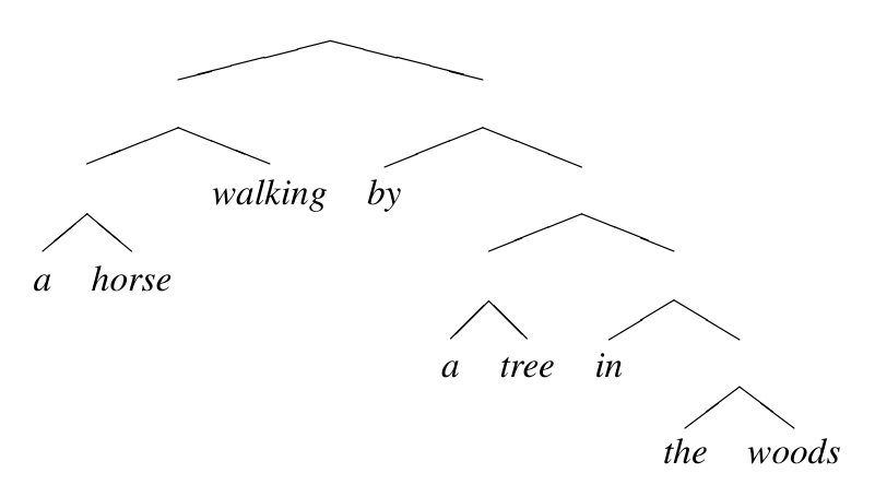
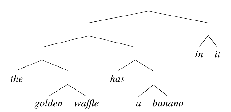
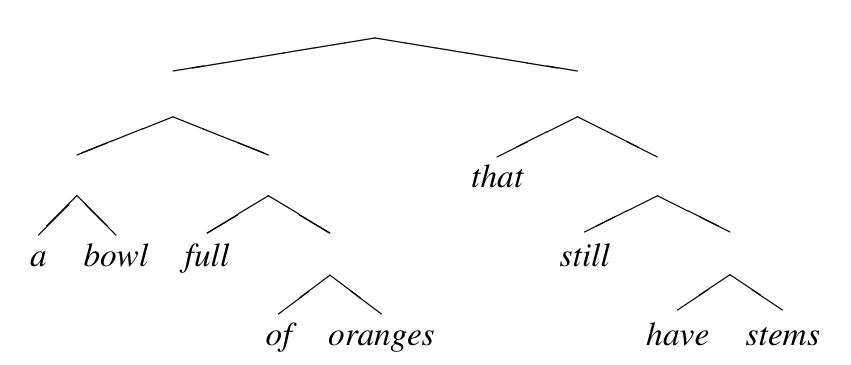
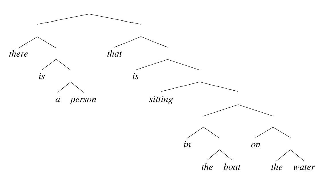
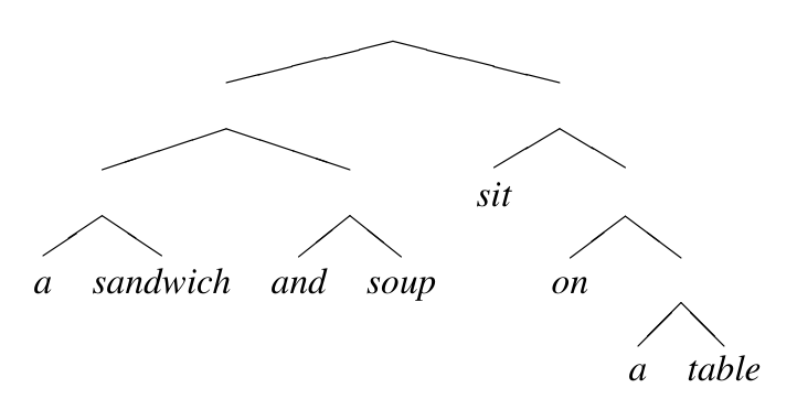
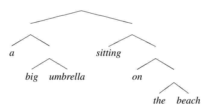
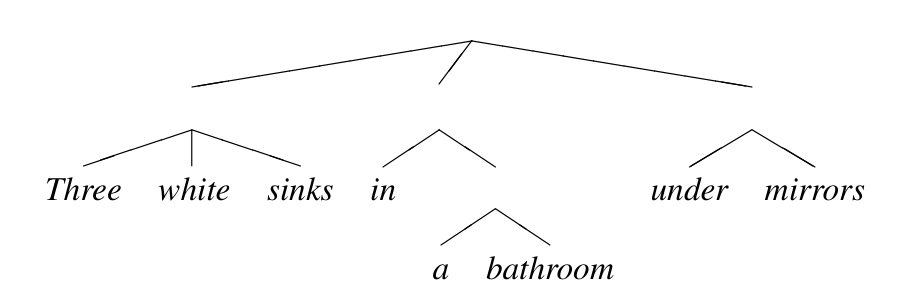
Figure 8 retains all eleven example trees across panels(a)–(k), including every word and branch. The captions come from the MSCOCO test set; these qualitative examples show the learned parser’s outputs, including imperfect or debatable attachments.